The P10 and ArCO2 data from Oct-Dec 2001 are reanalyzed and compared with simulated data from the gemsimulator package. The new analysis includes a study of a new track fitting algorithm.
The original fitting algorithm (Fit 1) was based on a naive chi**2 calculated by comparing the observed and model charge fractions in a row, and the standard deviation in the model fraction was fixed to be 0.05. There are two problems with this function: the standard deviations of model fractions depends on the primary electron statistics; the fractions in a row with only a few pads hit are highly (anti) correlated.
A new fitting algorithm (Fit 3) assumes that repeated measurements of charge fractions (for fixed track parameters) would yield a multinomial distribution, as defined by the primary electron statistics. Of course, the primary electrons are not directly counted... but we can assume that the fluctuations due to the amplification process and noise sources are small compared to the multinomial fluctuations. (This should be a good approximation given the rather large gains used). This method correctly accounts for correlations in a simple fashion. A small uniform probability for noise to occur is included, to avoid instability. The contribution to the likelihood for a simple multinomial distribution (for a single pad row) is given by:
npad
[Sum] n log(p ) + constant
i = 1 i i
Where n_i is the number of primary electrons "associated" with
a pad, and p_i is the model probability for a primary electron to
be associated with that pad. To estimate n_i, the GEM system gain
is used. With the noise term added, this changes to:
( p
+ p )
npad ( i noise )
[Sum] n log(---------------) + constant
i = 1 i (1 + npad p )
( noise)
In the following, plots are shown comparing: (Data, MC) x (P10, ArCO2) x (Fit1, Fit3).
| Run # | x0 (mm) | phi (rad) |
| 101 | 0. | 0. |
| 102 | 0.3 | 0. |
| 103 | 0.6 | 0. |
| 104 | 0.9 | 0. |
| 105 | 1.2 | 0. |
| 111 | 0. | 0.05 |
| 112 | 0.3 | 0.05 |
| 113 | 0.6 | 0.05 |
| 114 | 0.9 | 0.05 |
| 115 | 1.2 | 0.05 |
| 121 | 0. | 0.15 |
| 122 | 0.3 | 0.15 |
| 123 | 0.6 | 0.15 |
| 124 | 0.9 | 0.15 |
| 125 | 1.2 | 0.15 |
A sample of 2000 events (run 100) and 10000 events (run 110) was also generated with x0, phi, z0, and psi randomly selected. A corresponding set of runs were performed using P10 conditions using the run numbers in the 200's. The two .gem files can be found here: labArCO2.gem and labP10.gem. Two of the .gms files are here: run100.gmc and run200.gmc.
The rise time of the pulse depends, in principle, on the preamp specifications, on the drift velocity in the induction gap, the longitudinal extent of the charge cloud. One way to quantify the rise time is to look at the time required for the signal to rise from 50% (tr) to 100% (tp : peak time). The difference of these two times a function of tr is shown in this figure. To reduce the effect of induced pulses, the plot only includes pulses with amplitude at least 20 ADC counts. The data shows a much larger effect on the drift length than the MC. This may imply that longitudinal diffusion is not properly accounted for, but requires further study. Note that Magboltz calculations indicate that ArCO2 (90:10) should have less longitudinal diffusion than P10.
The full width half maximum of the pulses are shown here (again only those with amplitude of at least 20 ADC counts). Once again, the simulation is seen to be quite different from reality. A more sophisticated treatment of the time structure of the signals appears to be necessary.
The time structure is presently simulated in a simple way. The direct charge signal due to a single electron moving in the induction gap is assumed to follow a linear ramp function. To construct a signal due to a cloud of electrons the ramp function is convoluted with a gaussian, the standard deviation given by the standard deviation of arrival times at the pad. The calculations for this are shown here. The signals are then passed through a filter that simulates the rise time and fall times of the preamplifier electronics.
The resolution from fits to data was estimated by comparing the z0 estimate from 1 row to that with the 4 other rows. With simulated data, one can check that this procedure gives reasonable results. Since the simulated samples do not have the systematic effect discussed in the previous paragraph, they have better z resolution than the data samples.
The ntuples have the following variables relevant
to y-z tracking:
| variable | description |
| zb | the z0 estimate from a fit to all 5 rows in y-z (in ns) |
| zbxr(irow) | the z0 estimate from a fit to all rows except irow (in ns) |
| zbr(irow) | the z0 estimate from irow, fixing the angle psi from the zbxr fit (in ns) |
| z0mc | the true z0 for MC samples (in mm) |
The following table compares various resolution
estimates (in mm) from data and simulated samples:
| resolution estimate | P10 data | P10 MC (run 200) | ArCO2 data | ArCO2 MC (run 100) | comments |
| sigma of fit to (zbr-zbxr) (excluding tails) | 0.79 | 0.18 | 0.23 | 0.04 | to translate to single row resolution, divide by sqrt(1.25) |
| as above, limited to first 20 mm of drift | 0.74 +/- 0.06 | 0.18 | 0.11 | 0.04 | |
| sigma of fit to (zb-z0mc) (excluding tails) | 0.06 | 0.02 | to translate to single row resolution multiply by sqrt(5) ? | ||
| sigma of fit to (zbr-z0mc) (excluding tails) | 0.14 | 0.03 | single row resolution assuming fixed angle, psi |
Although the MC samples do not reproduce the data resolutions, the MC samples do indicate that the procedure for estimating the resolution works reasonably well.
The fitted values for sigma (the transverse size of the line charge) is shown for Fit 1 and Fit 3, and the data and MC are in reasonable agreement. The peaks at small values of sigma are due to some fitting pathologies, when there is little information to determine the sigma. These occur more frequently for ArCO2 data where the transverse diffusion is much less. There are fewer problematic fits when Fit 3 is applied, as compared to Fit 1.
The slope of sigma**2 vs drift time gives estimates
of the transverse diffusion in the drift volume, the intercept gives a measure
of the diffusion in the GEM itself.
| P10 data Fit 1 | P10 MC Fit 1 | P10 data Fit 3 | P10 MC Fit 3 | ArCO2 data Fit 1 | ArCO2 MC Fit 1 | ArCO2 data Fit 3 | ArCO2 MC Fit 3 | |
| A0 (mm^2) | -1.74 | -1.70 | -1.59 | -1.45 | 0.143 | 0.103 | 0.095 | 0.086 |
| A1 (mm^2/ns) | 0.00101 | 0.00102 | 0.00091 | 0.00086 | 0.31E-04 | 0.31E-04 | 0.34E-04 | 0.25E-04 |
| D (microns/sqrt(cm)) | 450 | 450 | 430 | 410 | 190 | 190 | 190 | 170 |
| D0 (microns) | 530 | 290 | 480 | 230 | 450 | 400 | 400 | 360 |
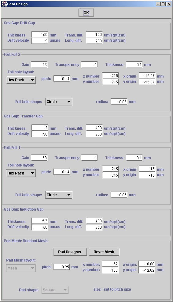
To estimate the diffusion constant, D, and the diffusion for zero drift, D0, it was assumed that the drift velocity for P10 and ArCO2 was 50 and 9 microns/ns. The time-zero (ie. zero drift) of the data is about 2000 ns, and for the MC is about 1750. The lack of precise knowledge of T0, results in large uncertainty in D0.
The actual diffusion constants used in the MC generation was 450 and 190 microns/sqrt(cm) for P10 and ArCO2 respectively. It appears that Fit 3 gives an estimate for the diffusion constant that is biased toward smaller values by about 5-10%. The transverse diffusion constant in the transfer and induction gaps (a total of 7.7 mm) was set to 450 and 400 microns/sqrt(cm). The latter value was inflated, from the Magboltz value of about 200 microns/sqrt(cm), to bring the observed diffusion in the GEM for ArCO2 to be closer to observed value.
Fit 1 does not include data from pads without signals above thresholds in calculating its chi**2. Fit 3 includes the information from all pads. Pad signals must be above a certain threshold (given by the parameter anmin) for them to included as a real signal in the pad fraction calculations. Pads with signals below the threshold level are assigned to have zero signal. The fact that Fit 3 does not account for the threshold requirement may explain why it underestimates the diffusion constant.
In analyses 1 and 2 estimates the x0 resolution in data were done by fitting x0,phi, and sigma with 4 rows and comparing the x0 value to a "fit" to x0 with the other row, keeping phi and sigma fixed at the result from the 4 row fit. With the MC data one can now check to see if that procedure gives a reasonable estimate for the single row position resolution.
The ntuples have the following variables relevant
to x-y tracking:
| variable | description |
| b | the x0 estimate from a fit to all 5 rows in xy (in mm) |
| be | the estimated uncertainty in b estimate (from delta chi**2 or Log Likelihood) |
| bxr(irow) | the x0 estimate from a fit to all rows except irow (in mm) |
| br(irow) | the x0 estimate from irow, fixing the angle phi and sigma from the bxr fit (in mm) |
| bxsr(irow) | the x0 estimate from a fit to x0 and phi using all rows except irow; sigma is calculated from drift distance |
| bsr(irow) | the x0 estimate from irow, fixing the angle phi and sigma from the bxsr fit |
| x0mc | the true x0 for MC samples (in mm) |
Fit 1:
| resolution estimator | P10 data | P10 MC | ArCO2 data | ArCO2 MC | comments |
| sigma of fit to (br - bxr) (excluding tails) | 400 | 310 | - | - | - : not gaussian |
| as above, limited to first 20 mm of drift | 250 | 190 | - | - | |
| sigma of fit to (bsr-bxsr) (excluding tails) | 400 | 310 | 320 | 230 | |
| as above limited to first 20 mm of drift | 250 | 230 | 220 | - | - : not gaussian |
| sigma of fit to (b-x0mc) | 90 | 60 | multiply by sqrt(5) to get single row resolution | ||
| as above limited to first 20 mm of drift | 50 | 50 | |||
| sigma of fit to (br-x0mc) | 260 | 190 | |||
| as above limited to first 20 mm of drift | 200 | 170 | |||
| sigma of fit to (bsr-x0mc) | 270 | 180 | |||
| as above limited to first 20 mm of drift | 170 | 130 | |||
| average be | 70 | 50 | |||
| as above limited to first 20 mm of drift | 50 | 50 * | * : not well behaved | ||
| sigma of fit to (b-x0mc)/be | 1.6 | 1.5 | error is underestimated |
Fit 3:
| resolution estimator | P10 data | P10 MC | ArCO2 data | ArCO2 MC | comments |
| sigma of fit to (br - bxr) (excluding tails) | 400 | 290 | - | - | divide by sqrt(1.25) to get single row resolution |
| as above, limited to first 20 mm of drift | 250 | 190 | - | - | " |
| sigma of fit to (bsr-bxsr) (excluding tails) | 400 | 290 | 270 | 220 | " |
| as above limited to first 20 mm of drift | 250 | 200 | 240 | 180 * | " * not gaussian |
| sigma of fit to (b-x0mc) (excluding tails) | 80 | 60 | multiply by sqrt(5) to get single row resolution | ||
| as above limited to first 20 mm of drift | 50 | 50 | multiply by sqrt(5) -> 110 microns | ||
| sigma of fit to (br-x0mc) | 260 | 180 | |||
| as above limited to first 20 mm of drift | 200 | 150 * | |||
| sigma of fit to (bsr-x0mc) | 250 | 160 | |||
| as above limited to first 20 mm of drift | 170 | 130 * | |||
| average be | 95 | 90 | 70 | 60 | |
| as above limited to first 20 mm of drift | 65 | 60 | 60 | 60 | |
| sigma of fit to (b-x0mc)/be | 1.1 | 1.0 | error is reasonably well estimated |
The following summarizes the important points from the study above:
The MC samples appear to simulate the x-resolution properties fairly well. This figure compares the distributions of (bsr-bxsr) for data(red) and MC(black) for Fit 3.
The MC samples confirm that the simple linear centroid method does much worse in determining the x coordinate for each row. This figure compares the residual for the centroid method (ntuple variable bl, in red) with the bsr method (in black) for the ArCO2 sample with z < 20 mm.
The uncertainties in the phi angle (phie) from the data and MC fits are 14 and 13 mrad, respectively.
The poor track fits occur more frequently in the CO2 data, because there are more pad rows with only a single hit, due to the lower transverse diffusion. The MC does not simulate this aspect very well: This figure compares the fraction of rows with only 1 pad hit for data and MC and for the two gas mixtures.
z < 10 mm
| 0 < phi < 0.05 | 0.05 < phi < 0.15 | 0.15 < phi < 0.35 | |
| Data | 211 +/- 28 | 229 +/- 18 | 266 +/- 28 |
| MC | 217 +/- 17 | 221 +/- 15 | 255 +/- 15 |
10 < z < 30 mm
| 0 < phi < 0.05 | 0.05 < phi < 0.15 | 0.15 < phi < 0.35 | |
| Data | 175 +/- 10 | 219 +/- 8 | 330 +/- 22 |
| MC | 176 +/- 8 | 188 +/- 7 | 228 +/- 9 |
The MC samples follow the same pattern as the data, showing an increase in the standard deviations for larger track angles. The MC only shows significant increase for the largest phi bin.
Using the MC samples, one can directly examine the residual distribution for x0 for different phi bins. This is shown in this figure for ArCO2 and this figure for P10, for drift distances less than 50 mm. The results for the standard deviations (in microns) are shown in the table below:
z0mc < 50 mm
| 0 < phi < 0.05 | 0.05 < phi < 0.15 | 0.15 < phi < 0.35 | |
| ArCO2 | 48 +/- 4 | 53 +/- 3 | 92 +/- 6 |
| P10 | 57 +/- 3 | 63 +/- 3 | 104 +/- 8 |
All of this suggests that there is not expected to be a significant track angle effect except for the largest phi bin.