GEM Simulation Studies

Updates:

• October 13: an error found in the simulation - longitudinal diffusion coefficient was used in place of the transverse diffusion coefficient. Replaced study with comparison to October 10 data (which used premix P10), instead of uncertain mix of Ar C0₂ from August data.

Program description

The program allows the user to design a GEM by placing components one on top of another. When single electrons or clouds of electrons are inserted in the GEM, the electrons propagate through all the GEM components, and signals are read from the GEM pads. Electrons drift in the -z direction, perpendicular to the layers of GEM components.

The components that make up a GEM are the following:

• A GEM foil; an array of holes in a thin sheet. The array can be either a grid or a hexagonal closed pack structure of circular or square holes.
• A pad array. This is the readout structure for a GEM. The pads, either circular or square, can be arranged on a grid or a hexagonal closed pack array. The pads are connected to readout electronics which are connected to a virtual scope that allows information about events to be graphically displayed. A statistics windows keeps track of important information from the pads for a given event or a run. Multiple pad arrays can be placed in the GEM to observe the development of the electron cloud as it moves through the GEM.
• A gas gap. This is the volume of gas that separates the foils and the pad arrays.

The electron propagation through the GEM parts is done with simple algorithms. Electrons are objects with space and time coordinates. When the electron moves through a gas gap, its time is incremented by the drift time. The drift time is the distance to the bottom of the gas volume divided by the drift velocity. To account for longitudinal diffusion, the drift time is smeared by a Gaussian with width given by sig_z/v_drift. where sig_z is given by sqrt(2 D_long t_drift), and D_long is the longitudinal diffusion coefficient. The electron x and y coordinates are smeared with a Gaussian whose width is determined from the transverse diffusion coefficient and its drift time. When an electron reaches a foil, it moves to the closest hole, and a Poisson number (with mean given by gain-1) of new electrons is produced at random locations within the hole. When an electron reaches a pad Array,  the electron is assigned to the nearest pad. For each pad, the mean and rms space-time coordinates for electrons originating from each primary electron is accumulated separately, to be used to define the signal shape once all electrons have been propagated through the GEM. In this way, the individual space-time coordinates millions of electrons produced do not have to be kept in memory.

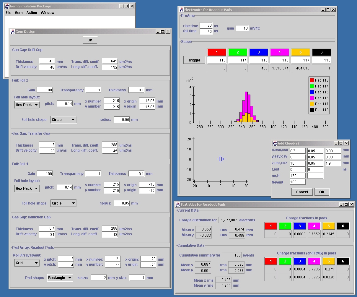
A screen shot of the program, with the default parameters used in the simulation are shown in the figure linked here.  The window entitled, Gem Design, shows all the parameters that can be adjusted for the Gem. Additional GEM components are added to this window by selecting the menu item in the main Gem Simulation Package window. Data were collected for a set of 100 events, each event consisting of a cloud of 170 primary electrons, producing 1.7M secondary electrons. The electronics window shows, for the last event, the arrival times for electrons at the pads and a "box style" distribution of the hits on the pads. The statistics window shows some information about the last event (upper part) and summary information for all 100 events (lower part).

At this time, the program does not simulate pulse shapes. Its first application is to study the intrinsic resolution from charge sharing.

Download

Simulation studies

Clouds are formed from 170 electrons, with the electrons distributed about the cloud centre according to a 3D Gaussian with 50 microns standard deviation in all three directions. The cloud centres are distributed uniformly in z in the drift gap region and spread out in x and y about the coordinate (0.7, 0.0) by a Gaussian distribution of 30 microns. The value of 30 microns comes from the following considerations:

• collimator spot size: diameter 50 microns. The projection of a circle onto the x axis gives a distribution with mean 0 and standard deviation of r/2, or 12.5 microns for a 50 diameter spot size. The spot size may be larger since the collimator hole is some distance from the drift gap.
• range of knock on and Auger electrons might add an rms of 30 microns.

For the 100 events, the centre pad collected, on average, 0.729 of all of the charge, with an RMS of 0.0226. One can use this information along with the known position of the cloud centre and pad boundary to determine the size of the cloud and the resolution of the position coordinate, just as it was done in the data analysis. The method, however, is much simpler with rectangular geometry as one only needs to integrate a Gaussian in one dimension. For this case, the integral of a Gaussian from -infinity to +0.608 sigma yields 0.729. Therefore, the pad boundary (at x=1 mm) is located at 0.608 sigma away from the cloud centre (at x=0.7 mm). Hence, the width of the charge distribution is given by 0.3/0.608 = 0.493 mm, which is about the same value as determined by looking at the statistics of all of the electrons.

The RMS of 0.0226 corresponds to a variation in the upper limit of the Gaussian integral of 0.070 sigma. Therefore the spread of centroid measurements from this data would be about 34 microns. This spread of measurements is what we have called resolution in the data analysis. For this simulation, the spread has the dominant contribution coming from the width of the distribution of primary electron cloud centres (30 microns) and does not reflect the intrinsic resolution of the device.

The spread of the position measurements observed in the two analyses (#2 and #3)  for the two gas mixtures is approximately 50 microns. Since the two gas mixtures (ArC0₂ and P10) have very different transverse diffusion, it appears that the diffusion is not a dominant factor in the measurement spreads. To bring the simulation into better agreement with the data, the sigma in x and y of the cloud centres was increased as shown in the table below. Each row represent the results from a run of 100 events, and it appears with those statistics the measurement spread is determined only to within 10%.
 
 

For the simulation studies shown below, the beam widths are set to 50 microns in x and y.

Contribution to measurement spread from cloud size variation

The contribution from diffusion is well parametrized by the size of the cloud as it crosses the top foil divided by the square root of the number of primary electrons. The size of the cloud at that point is found by adding a "virtual" pad array just above foil 2.  The entries in the tables below correspond to runs of 10 events each.
 
 

The simulation finds that the cloud sizes range from 444 - 549 microns, in agreement with the rough determination from data of 50 microns for the standard deviation of the cloud widths.

The 4th column shows that the average diffusion does not contribute significantly to the measurement spread. The fact that different events have different diffusion generated cloud sizes, however, does contribute to the measurement spread for events away from the pad boundaries.
 
 
 
 

To be continued...