The data runs are summarized below. The collimator
location is indicated using the coordinate system described above.
| run number | x_coll (mm) | y_coll (mm) |
| 1001 | 0. | 1.443 |
| 1002 | 0. | 1.543 |
| 1003 | 0. | 1.243 |
| 1004 | 0. | 1.043 |
| 1005 | 0. | 0.843 |
| 1006 | 0. | 0.643 |
| 1007 | 0. | 0.443 |
| 1008 | 0. | 0.043 |
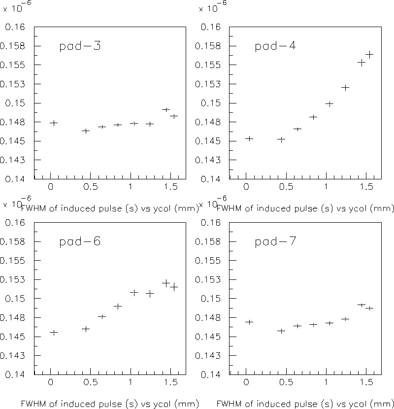
If the gain variation was due to changes in gas composition, then there might be a visible change in the drift velocity. This would, in turn, change the width of the induced pulses, since the full width of these pulses is just the drift time across the GEM induction gap. The FWHM of induced signals in pads 3,4,6, and 7 do show variations in the pulse width, but the variations are not consistent from one pad to another and therefore cannot be attributed to changes in drift velocity. Just as in the 2nd analysis, the variations are largest in pad 4. This may indicate a problem in the electronics for channel 4 downstream of the preamps.
The GEM position analysis uses ratios of peak voltages, so the run-to-run gain variation should have a small effect, provided that pedestals are properly accounted for. However, if the pads do not have equal gains, then this could cause difficulties. A future data set should include calibration runs where the x-ray collimator is on runs where the x-ray collimator is placed roughly over the centre of each of the 7 pads under study.
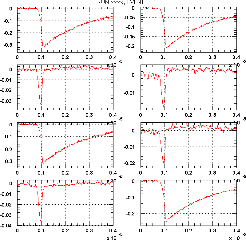
The figure linked here shows data from a typical event, after pedestal correction, when the x-ray collimator was positioned over the coordinate (0.,1.243) (mm). Note that the baselines for the induced pulses in pads 4 and 6 are not zero, after the induced pulses. These baseline shifts unfortunately are not constant from one run to the next. The size of these shifts (of order 1 mV) correspond to the scale of changes in the induced signals that result when the x-ray pulse is moved 100 microns, so this effect is important to understand (and to reduce as much as possible in future data taking).
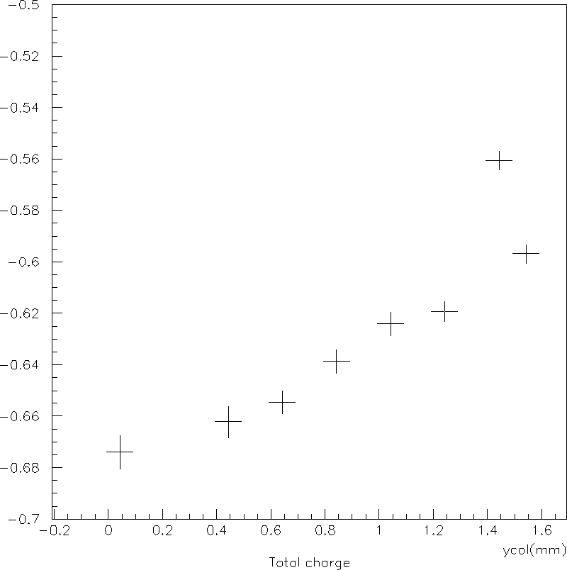
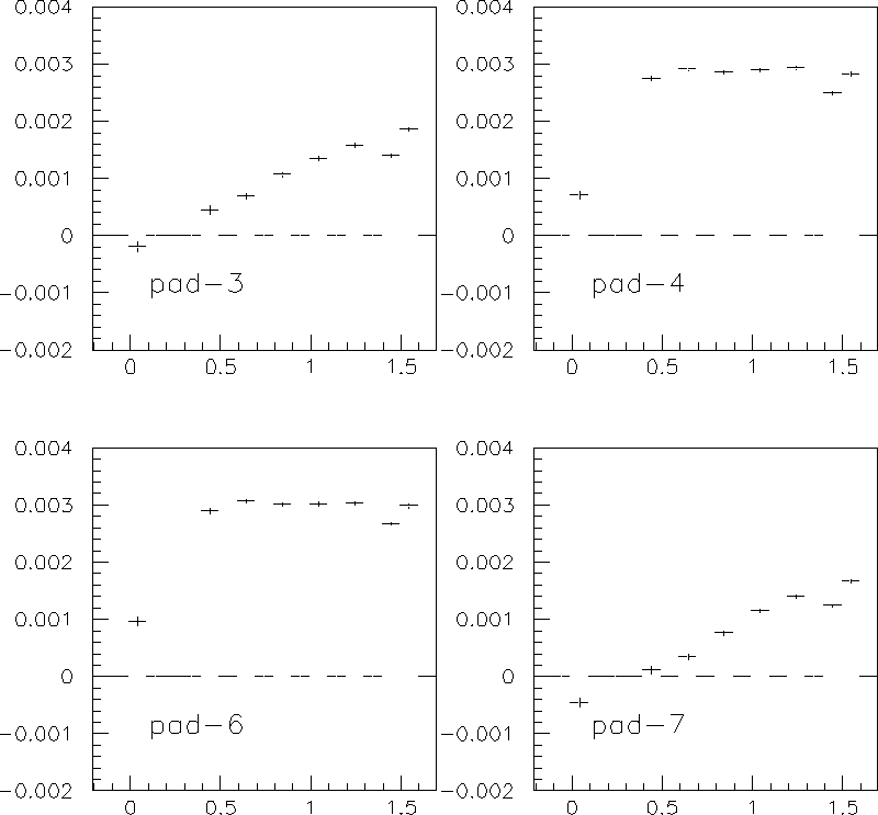
Some plots have been produced to characterize the baseline changes: The pulse shape is fit to a quadratic 600ns - 1800 ns after the induced pulse. The value of the fit at the point 1200 ns after the pulse defines the "baseline". The value of the baseline for the different runs are shown in the figure linked here. The baseline in pads 4 and 6 are roughly constant for ycol > 0.4 mm but reduces for ycol = 0.043. The baseline in pads 3 and 7 reduce smoothly as the collimator moves closer to the centre of pad 1. Unlike the 2nd analysis, the variation is consistent with a small amount of charge sharing: pads 4 and 7 behave similarly as do pads 3 and 6. There appears to be a constant positive offset of about 3 mV (overshoot from electronics?) that is canceled by varying degrees by some small direct charge component. As the x-ray collimator moves closer to the pad, more charge is deposited on the pad and the cancellation becomes larger.
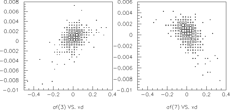
The hypothesis that the baseline variation is due to charge sharing is confirmed by looking at how the baseline is related to the x coordinate of the individual events (determined through the charge sharing from pads 1,2, and 8). The figure linked here, shows the scatter plot of the baselines vs. x coordinate of the x-ray absorption, for pads 3 and 7 for run 1006. Events with x-rays closer to pad 3 have more negative baselines for that pad, and a less negative baselines for pad 7.
Unlike the previous analysis there is no evidence for crosstalk between channels. Whereas in the previous analysis, the baseline in pad 4 was strongly correlated to the amplitude of the pulse in pad 2, this data sample has the the baseline in pad 4 roughly constant for a wide range of y-collimator positions (and therefore a wide range of pulse amplitudes in pad 2). The most likely explanation is that the cross talk originated in the HQV810 preamplifier cards.
Note that because there are multiple changes compared to the previous data set, one cannot be certain that the cross talk seen in the 2nd analysis is not present here. Because of the change in the scope time division, the baseline measurement is taking place much later (1200 ns after the pulse) than in the 2nd analysis (300 ns after the pulse).
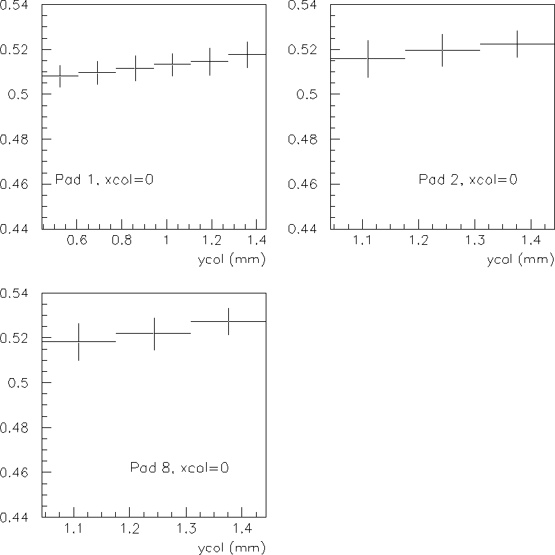
The figure linked here shows the mean ratio of the "late" to the peak amplitudes on pads 1,2, and 8 for different collimator positions. The error bars indicate the standard deviations of the ratio. (The mean and standard deviations are found by fitting each ratio distribution to a Gaussian). Since the standard deviation is less than 1%, the late amplitude is used instead of the peak amplitude for the charge fraction determination of both direct and mixed signals. The ratios differ for pads 1, 2, and 8, by only about 2%. In the 2nd analysis, the ratios differed by 6%, presumably due to slightly different time constants in the readout electronics.
AN_pad = AF_pad / R_padwhere R_pad is the mean ratio of late to peak amplitudes, from the previous section. R_1 = 0.518, R_2 = 0.522, and R_8 = 0.527.
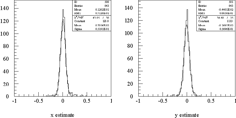
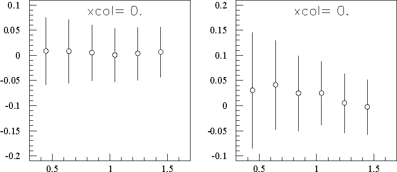
A summary for the x and y measurements for the runs is shown in the figure linked here. The left plot shows the mean and standard deviation of the x estimates, and the right plot shows the mean and standard deviation of the y estimates (with respect to the y collimator position). The right plot shows two new effects. There is a small bias in the measurement that grows as the collimator moves away from the 3 pad vertex. The second effect is that the standard deviation of estimates grows as the collimator moves away from the 3 pad vertex.
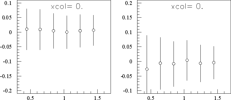
The first effect is easily corrected by increasing the size of the cloud in the model, from 0.53 mm (as determined above) to 0.56 mm. It is not clear why the determination above does not result in a bias free y coordinate measurement. The summary of the x and y measurements with this new cloud size is shown in the figure linked here.
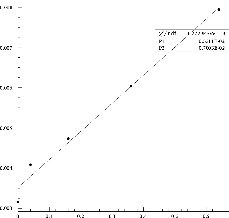
The observed increase in the spread is also consistent with this explanation. The variance of the measurements should be the sum of the variance due to non-diffusion effects and the variance due to the cloud size variation. The latter term scales as,
var(cloud size) = (fraction * displacement from vertex)**2
where "fraction" is the 1 standard deviation of the cloud widths divided by the mean cloud width. The variance of the y measurements is shown versus the square of the displacements from the vertex in the figure linked here, and is fit to a line. The fit result for "fraction" is sqrt(0.0070) = 0.084. In other words this model ascribes the additional spread due to cloud size variation, with the cloud size distribution having a mean of 560 microns and a standard deviation of about 50 microns.
Now to compare this to expectations: Since x-rays can be absorbed anywhere in the drift volume, the total drift length is between 8 and 12 mm. The cloud size scales like the square root of the total drift length. So cloud sizes would vary between 610 and 500, due to the different conversion points in the z direction. This is very similar to the standard deviation derived from the data above.
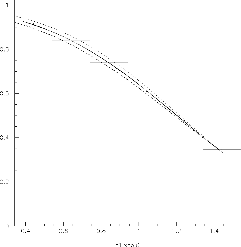
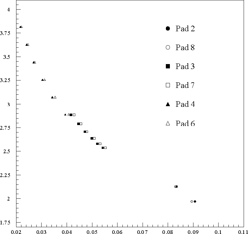
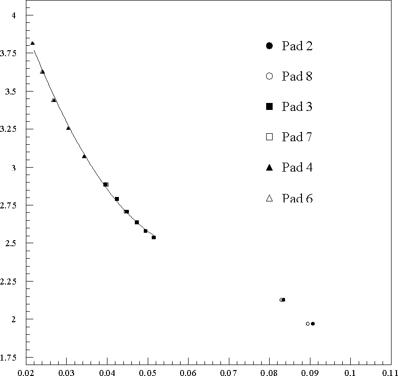
The data taken along the line (x=0) is used to characterize the induced response function. The ratio of the peak amplitude of the induced pulse to the total charge of the event is shown as a function of distance to the pad centre is shown in the figure linked here. The response function from the various pads do not perfectly line up. This is assumed to be due to unequal gains of the preamps, and so scaling factors (of order 5%) are applied to the observed pulse amplitudes (one for each each pad). This improves the agreement, as shown in the figure linked here, so that a universal pad response function can be used. This function defined by a 2nd order polynomial fit to the data, shown in the previous figure.
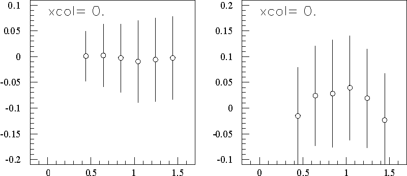
The summary of the x and y measurements are shown in the figure linked here. In the left plot, the vertical axis is the difference between the measured x location and the x location of the collimator (for this data xcol=0). The vertical bars represent the standard deviation as determined from fits of the data to Gaussians. The right figure is the same for the y coordinate measurement. There are some systematic biases in the y coordinate measurement of order 50 microns, which is not present for the x estimate. The 1 standard deviation spread in x measurements varies from 50 to 80 microns; for y measurements it is 90-100 microns. Unlike the charge sharing measurement, the spread in the y measurements does not depend strongly on the y collimator position.
The intrinsic position resolution of the GEM
devices therefore is even better than the 50-60 microns quoted by the 2nd
analysis.