A second analysis of 2D GEM position resolution
Dean Karlen / September 13, 2000
Index
- Gem pad layout
- Gem data
- Gem data analysis programs
- Gain variation
- Pedestals
- Separation of direct and induced components of signals
- Position analysis from direct charge sharing
- Determination of charge
- Observed charge fraction in pad 1 - determination of cloud size
- Determining position from charge fractions
- New method - Integration of Gaussians over hexagons
- Demonstration of new method with data
- Estimating the number of electrons in the cloud
- Summary of charge sharing results
- Position analysis from induced pulses
- Combination of charge sharing and induced measurements
- Conclusion
GEM pad layout
The figure linked here shows the assumed GEM layout and coordinate system. Dimensions are in mm. The pads are numbered from 1 to 8, according to the readout channel. The central pad is read out by both oscilloscopes (channels 1 and 5), to provide a common trigger. The coordinates of a few points are shown in colour.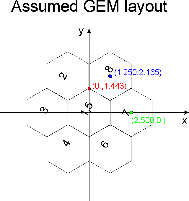
GEM data
The data sets taken during the period August 22-29 were taken with Ar-C02 (80-20) (110ml/min; 27.5ml/min) with Vdrift = 4000V, and Vgem=3600V, using the HQV810 preamplifier, and the xray tube set at 6 kV. About 1000 events are taken for each run.The data runs are summarized below. The first
two digits of the run number correspond to the day of August that the data
was taken. The collimator location is indicated using the coordinate system
described above.
| run number | x_coll (mm) | y_coll (mm) |
| 2201 | 0. | 1.443 |
| 2202 | 0. | 1.543 |
| 2203 | 0. | 1.643 |
| 2204 | 0. | 1.343 |
| 2205 | 0. | 1.243 |
| 2206 | 0. | 1.143 |
| 2207 | 0. | 1.043 |
| 2208 | 0. | 0.943 |
| 2209 | 0. | 0.843 |
| 2210 | 0. | 0.743 |
| 2211 | 0. | 0.643 |
| 2212 | 0. | 0.543 |
| 2213 | 0. | 0.443 |
| 2214 | 0. | 0.343 |
| 2215 | 0. | 0.243 |
| 2301 | 0. | 0.143 |
| 2302 | 0. | 0.043 |
| 2401 | 0. | 0. |
| 2402 | 0. | -0.057 |
| 2403 | 0. | -0.157 |
| 2404 | -0.100 | -0.157 |
| 2405 | -0.100 | -0.057 |
| 2406 | -0.100 | 0.043 |
| 2407 | -0.100 | 0.143 |
| 2408 | -0.100 | 0.243 |
| 2409 | -0.100 | 0.343 |
| 2501 | -0.100 | 0.443 |
| 2502 | -0.100 | 0.543 |
| 2503 | -0.100 | 0.643 |
| 2504 | -0.100 | 0.743 |
| 2505 | -0.100 | 0.843 |
| 2506 | -0.100 | 0.943 |
| 2507 | -0.100 | 1.043 |
| 2508 | -0.100 | 1.143 |
| 2509 | -0.100 | 1.243 |
| 2801 | -0.100 | 1.343 |
| 2802 | -0.100 | 1.443 |
| 2803 | -0.100 | 1.543 |
| 2804 | -0.200 | 1.543 |
| 2805 | -0.200 | 1.443 |
| 2806 | -0.200 | 1.343 |
| 2807 | -0.200 | 1.243 |
| 2808 | -0.200 | 1.143 |
| 2809 | -0.200 | 1.043 |
| 2810 | -0.200 | 0.943 |
| 2811 | -0.200 | 0.843 |
| 2812 | -0.200 | 0.743 |
| 2813 | -0.200 | 0.643 |
| 2814 | -0.200 | 0.543 |
| 2815 | -0.200 | 0.443 |
| 2816 | -0.200 | 0.343 |
| 2817 | -0.200 | 0.243 |
| 2818 | -0.200 | 0.143 |
| 2819 | -0.200 | 0.043 |
| 2820 | -0.200 | -0.057 |
| 2901 | -0.300 | 1.443 |
| 2902 | -0.300 | 1.343 |
| 2903 | -0.300 | 1.243 |
| 2904 | -0.300 | 1.143 |
GEM data analysis programs
The results shown below come from the gemanal program (version 0.7) located in the directory /home/karlen/gem. An associated paw kumac file, gemanal.kumac, is found in the same area.Gain variation
The gain of the system is constant over these runs only to within about 20%, as can be seen in the figure linked here. This figure shows the the sum of peaks seen in the 3 pads (1,2,8). Large steps occur within the days' sets of runs on August 22, 24, and 25. It would be helpful to understand the source of these changes. Looking at the gradual changes in the gain, there appears to be a general tendency for the peak value to decrease as the collimator moves towards the centre of pad 1. This may be an indication that the gain of the system over the central pad may be somewhat less than that over the other two pads. The centring of the collimator over the vertex of the three pads assumes that the gain of the system is uniform over the entire gem.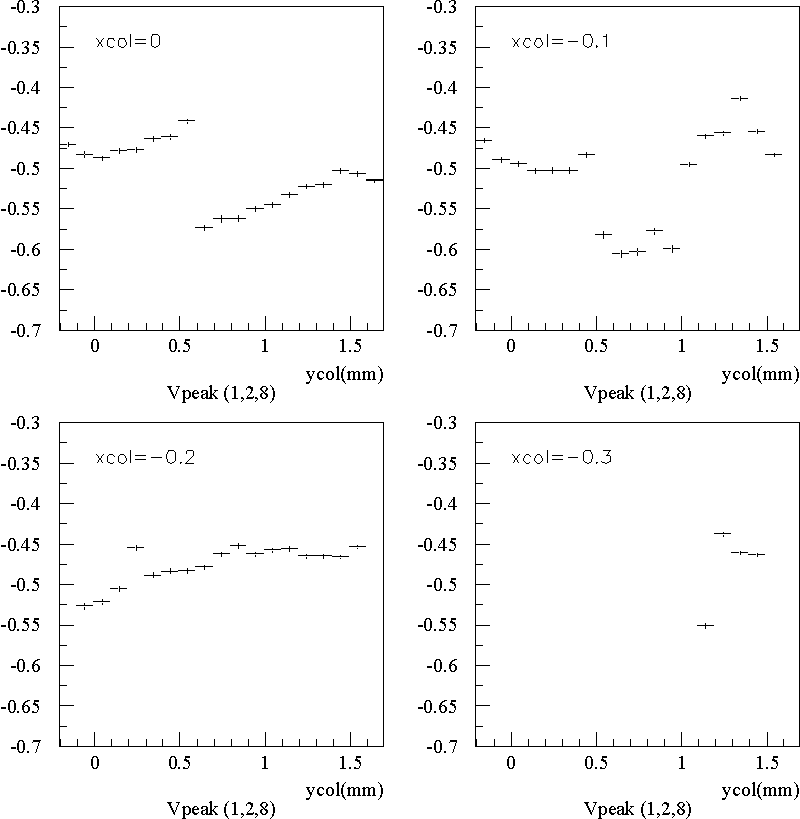
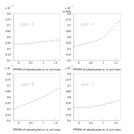
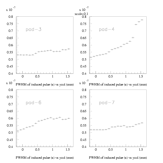
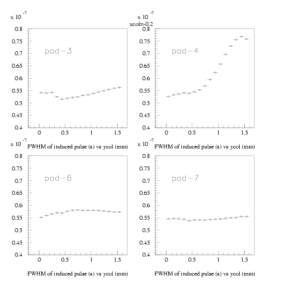
If the gain variation was due to changes in gas composition, then there might be a visible change in the drift velocity. This would, in turn, change the width of the induced pulses, since the full width of these pulses is just the drift time across the GEM induction gap. The FWHM of induced signals in pads 3,4,6, and 7 for xcol=0, -0.1, and -0.2, do show variations in the pulse width, but the variations are not consistent from one pad to another and therefore cannot be attributed to changes in drift velocity. The variations are largest in pad 4. As shown in the next section, this pad suffers signifigant cross talk with pad 2, and therefore the observed changes in the pulse widths may be due to this effect.
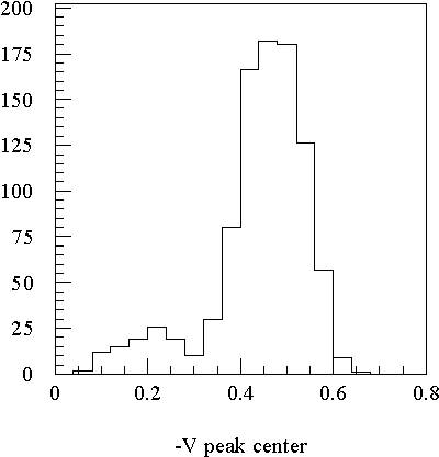
The spectrum for run 2401, when the collimator was located at (0.,0.), is shown in the figure linked here. A small escape peak appears to be present.
The GEM position analysis uses ratios of peak voltages, so the run-to-run gain variation should have a small effect, provided that pedestals are properly accounted for. However, if the pads do not have equal gains, then this could cause difficulties. A future data set should include calibration runs where the x-ray collimator is placed roughly over the centre of each of the 7 pads under study.
Pedestals
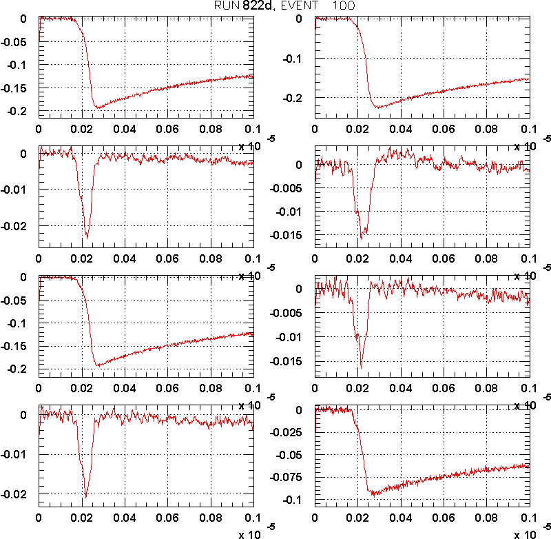
The data for each channel is corrected by using a pedestal defined by the average of measurements before the pulse (time bins 10-60). There are, however, baseline shifts that remain after this correction.The figure linked here shows data from a typical event, after pedestal correction, when the x-ray collimator was positioned over the coordinate (0.,1.343) (mm). Note that the baselines for the induced pulses in pads 3,4, and 7, are not zero, after the induced pulses. These baseline shifts unfortunately are not constant from one run to the next. The size of these shifts (of order 1 mV) correspond to the scale of changes in the induced signals that result when the x-ray pulse is moved 100 microns, so this effect is important to understand (and to reduce as much as possible in future data taking).
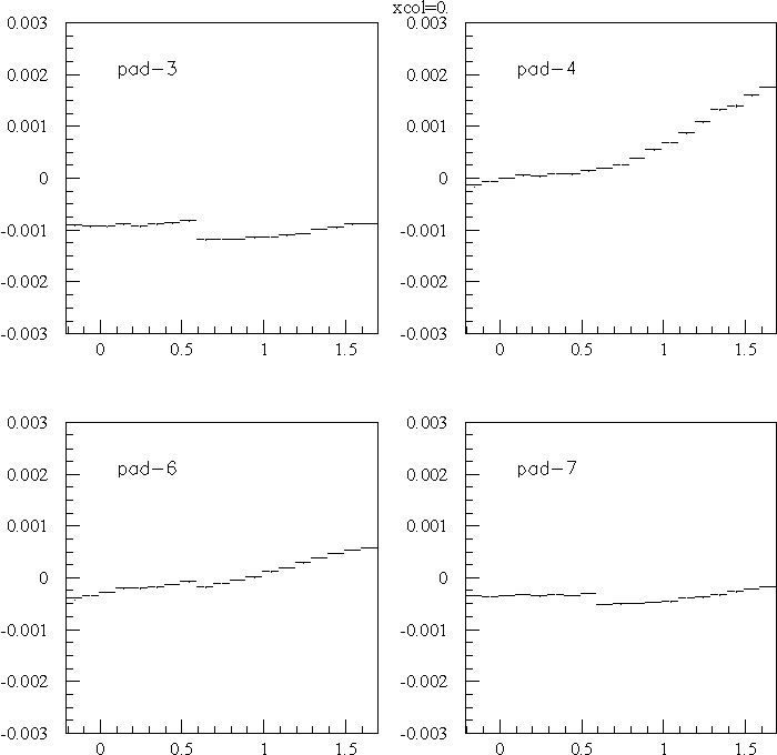
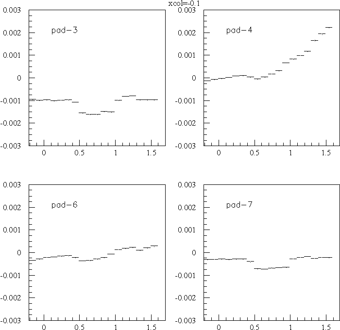
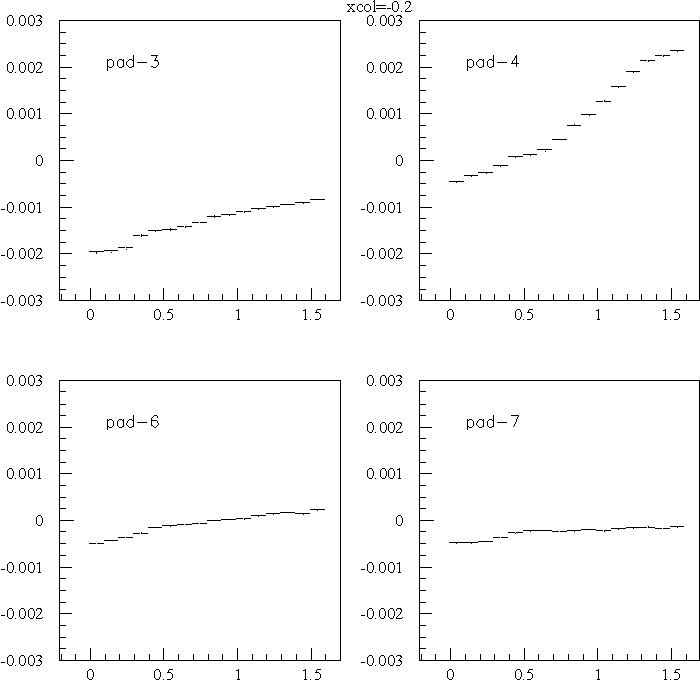
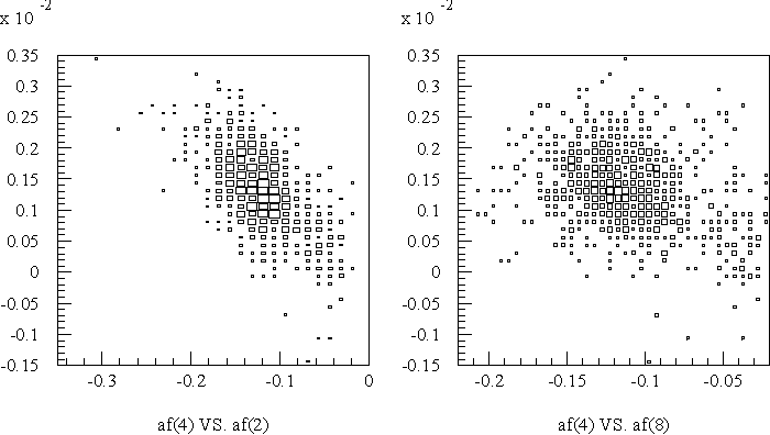
Some plots have been produced to characterize the baseline changes: The pulse shape is fit to a quadratic 150ns - 450 ns after the induced pulse. The value of the fit at the point 300 ns after the pulse defines the "baseline". The value of the baseline from run to run are shown for xcol = 0., -0.1, and -0.2. Pad 4 shows the largest variation in baseline. This variation is inconsistent with being due to a small amount of charge sharing, since one would not expect to see the fastest variation when the x-rays are furthest away from the pad. As well, baseline variation in pad 6 does not show the same behaviour. It appears that Pad 4 may be picking up some cross talk from pad 2. The baseline variation for pad 4 drops to zero as the x-rays move far enough away from pad 2, that it no longer collects any direct charge. The figure linked here shows that in run 2204 there is a strong correlation between the baselines in pad 4 and 2, as compared to no correlation in the baselines between pads pads 4 and 8. This almost certainly indicates the baseline variation is in fact due to crosstalk.
The varying pedestals (due to cross talk) and varying gains (probably due to changes in gas properties) make the analysis of this data set more complex. There are no repeated data samples (at the same collimator location) that could help determine the optimal method to account for gain and pedestal variation.
Afterwards, Jacques Dubeau did a study of cross talk in the HQV810. See the page linked here.
For future data runs, if the gain and pedestals cannot be held constant, then it is will be useful to take several runs at some reference location (interspersed amongst runs at other locations).
Separation of direct and induced components of signals
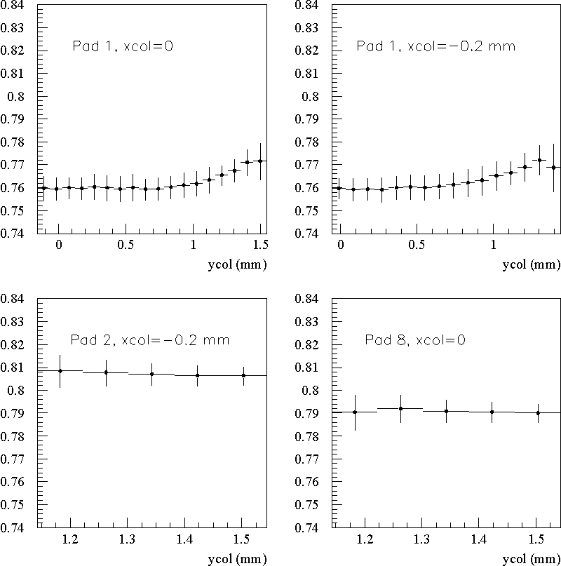
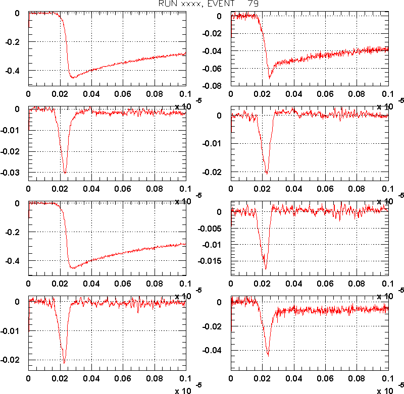
There are three categories of signals observed: Pads that collect a large fraction of the charge have signals with a large decay time, and are called "direct signals". Signals on pads that do not collect charge quickly return to zero are called "induced signals". The third category are those which have a significant component due to both direct and induced components. Pulses belonging to the last category are called "mixed signals", and it is useful to be able to determine what fraction of a mixed signal is due to direct charge.To deduce the direct component of a signal, the pulse is fit 300 ns after the peak occurs. For induced signals this "late" amplitude is near zero, apart from the baseline shifts described above. For pad 1, where the signals always have a large direct charge component, the ratio of this "late" amplitude to the peak amplitude is independent of the peak amplitude and of the location of x-ray collimator. Therefore, the "late" amplitude can be scaled to estimate with good precision the size of the direct charge component in a mixed signal.
The figure linked here shows the mean ratio of the "late" to the peak amplitudes on pads 1,2, and 8 for different collimator positions. The error bars indicate the standard deviations of the ratio. (The mean and standard deviations are found by fitting each ratio distribution to a Gaussian). Since the standard deviation is less than 1%, the late amplitude is used instead of the peak amplitude for the charge fraction determination of both direct and mixed signals. The mean ratio is different for pads 1, 2, and 8, presumably due to slightly different time constants in the readout electronics for these pads.
The use of the late amplitude for direct charge determination is much simpler than attempting to fit the mixed signals for direct and induced components.
Position analysis from direct charge sharing
Determination of charge
The data from these runs were used to map out the pad response function for direct charge collection. The charge collected by a pad is assumed to be proportional to the peak amplitude of the pulse for signals dominated by direct charge collection. Rather than use the peak amplitude (VP) directly, the "late" amplitude (AF) is used, and scaled to a new value (AN) corresponding to the peak amplitude, as follows:AN_pad = AF_pad / R_padwhere R_pad is the mean ratio of late to peak amplitudes, from the previous section. R_1 = 0.760, R_2 = 0.806, and R_8 = 0.790.
The total charge collected by all pads, determined this way, is shown in the figure linked here. The apparent gain variation from run to run on a given day is somewhat smaller than in the figure shown above, presumably because the total charge calculation is improved.
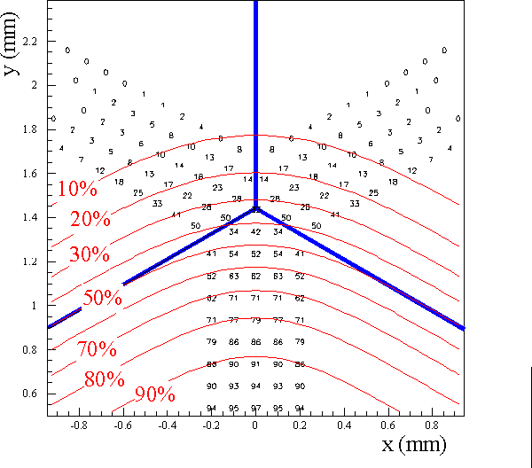
Observed charge fraction in pad 1 - determination of cloud size
The figure linked here shows the percentage of charge collected by pad 1, centred at (0,0), for various locations of the x-ray collimator. Symmetry was used to infer the values for pad 1 using the data from pads 2 and 8. The lines show the edges of the hexagonal pads. There are some anomalies near the edges of the pad 1. This may indicate an alignment error. [NOTE: The assumed positions of the collimators for these runs have since been determined to have been incorrect, as shown below.]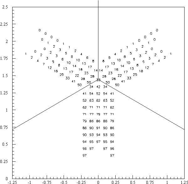
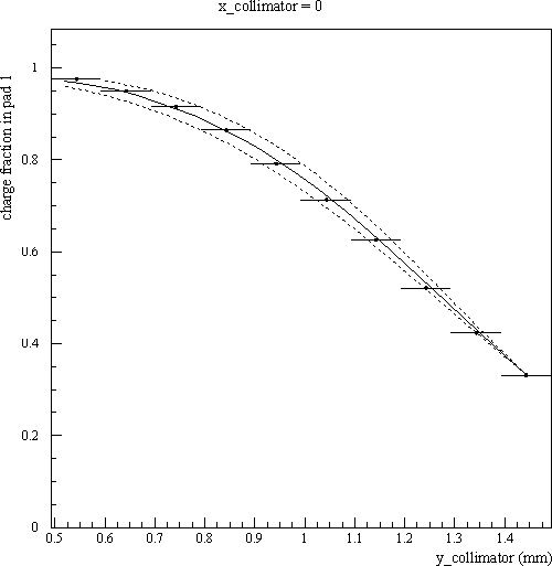
The data shown in the previous figure gives a direct indication of the transverse size of the charge distribution, which is expected to be primarily due to by diffusion. To quantify this, the probability density of charge is assumed to be a 2D Gaussian with sigma_x = sigma_y. The charge fraction expected in pad 1 in this model is found by integrating the 2D Gaussian over the hexagonal region defined by the pad. The integration is done numerically and is found to be in excellent agreement with the measurements. The figure linked here shows the observed charge fraction in pad 1, as a function of the y-coordinate of the collimator. The solid curve shows the prediction of the model when sigma_x=0.37 mm. The dashed curves show the predictions for sigma_x = 0.34 and 0.40 mm. By eye it appears that sigma_x can be determined to better than 10 microns. Note that sigma_r = sqrt(2) sigma_x. According to this model, diffusion leads to an effective cloud size of sigma_r = 0.52 mm. If the diffusion was the only contribution, with 150 electrons per primary x-ray, the diffusion limit to the position resolution in x or y would be about 30 microns.
Determining position from charge fractions
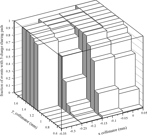
The method of determining the position, by a "centre of mass" technique was investigated in the first analysis. In this approach, the pad centre positions are weighted by a function of the charge fraction in each pad. The method was found to be successful for measurements along the symmetry line in which data was taken. It however had significant biases for points off that line. Linear weighting of the pad centres is not general enough to take into account the complex hexagonal geometry. As a result a more sophisticated method is used, and is described below.Since the charge cloud is much smaller than the pad size, at most three pads would be expected to share charge in any one event. For the analysis presented here, events are selected where pads 1, 2, and 8 (and only those pads) share significant charge. The selection criteria uses the fitted signal amplitude 300ns after the peak of the pulse. If that amplitude is below -10mV, the signal is considered for the charge sharing analysis. For example in this event, the signal in pad 2 passes the criteria, whereas the pad 8 signal does not. By demanding exactly 3 pads satisfy this criteria limits the region in the gem for which position can be estimated with this method. The figure linked here shows a 2D histogram showing the efficiency of this cut for different regions of the pad. The charge sharing technique can be used to determine the position only for x-rays within about 0.7 mm of a 3-pad vertex. For the set of collimators positions used in the runs analysed here, almost half of the events have exactly 3 pads passing the criteria.
New method - Integration of Gaussians over hexagons
A method for estimating the centroid of the charge distribution was developed by using a physical model, as opposed to empirical determination of weighting factors from data. The charge cloud is assumed to be in a shape of a 2D Gaussian and each pad is assumed to collect the charge from the cloud directly over it. With this model, the fraction of charge collected by each pad (the so-called pad response function) can be predicted as a function of the offset (v) of the 3-pad vertex from the cloud centroid, by integrating the 2D Gaussian over the pad regions. A picture describing the model is linked here. The Gaussian is shown in red, the pads are shown in blue. There is a unique combination of charge fractions in each pad for each vector, v. Using data from this model, the inverse of the pad response function (ie. a 2D mapping from 2 charge fractions to the two coordinates of v) is derived.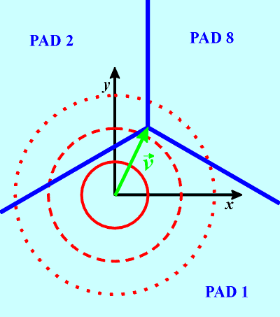
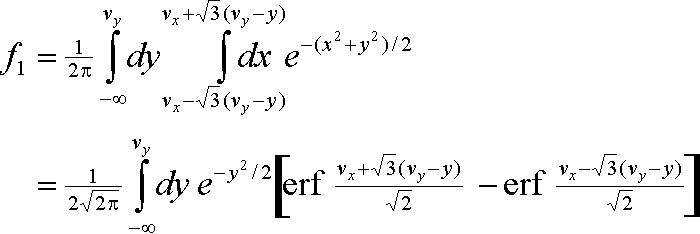
Details of the calculation are given here. The fraction of charge in pad 1, f1, is
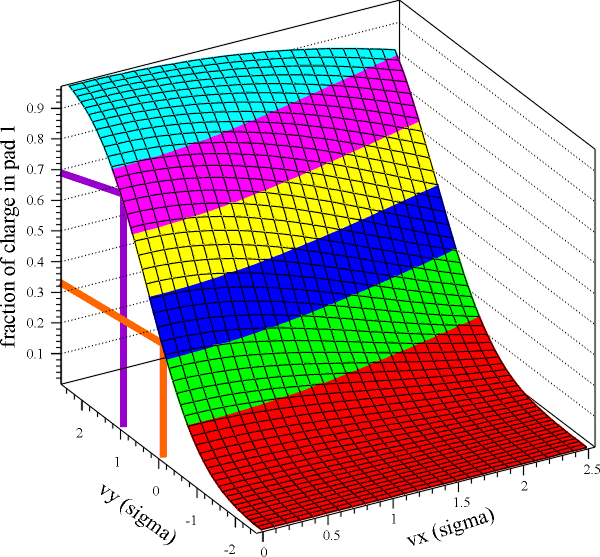
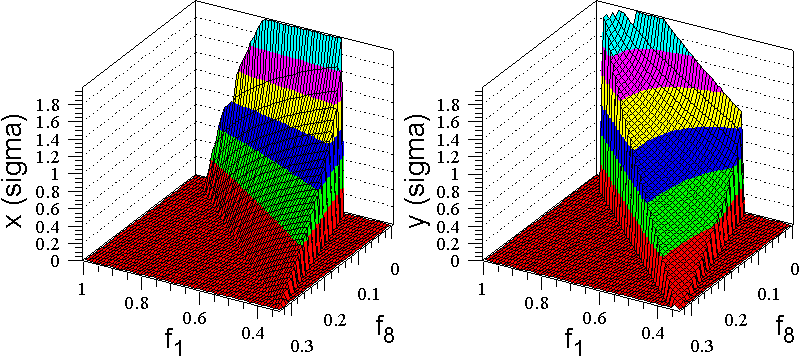
No simplification of the second integral has been found, so it is evaluated numerically. The fractions in the other two pads, f2 and f8, can be found by a rotation of coordinates. A plot of this function is given in the figure linked here. In this figure, the displacement vector components are given in units of standard deviations of the cloud. The charge fraction of 0.33 for a cloud centred over the 3-pad vertex is read from the plot by following the orange lines. The purple lines show the charge fraction of 0.69 when the 3-pad vertex is displaced by 1 sigma in the y direction with respect to the 3-pad vertex.
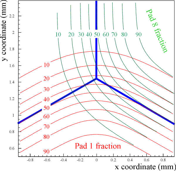
The function can be superimposed on the measurements for f1, presented above. The value of sigma is taken to be 0.370 mm, and the contour of the function is overlaid on the data in the figure linked here. The figure linked here overlays both the f1 and f8 contours in the GEM coordinate system.
The joint inverse of the functions f1 and f8 gives the necessary information to convert charge fractions to x-ray coordinates. These functions, vx(f1,f8) and vy(f1,f8), are tabulated by sampling the f1 and f8 functions at various offsets. The values, vx and vy, are found by linear interpolation of the tabulated values. These are then converted to the GEM coordinate system.
This method has only one free parameter, the average cloud size. There are no other constants derived from the data in the calculation of the x-ray location.
Demonstration of new method with data
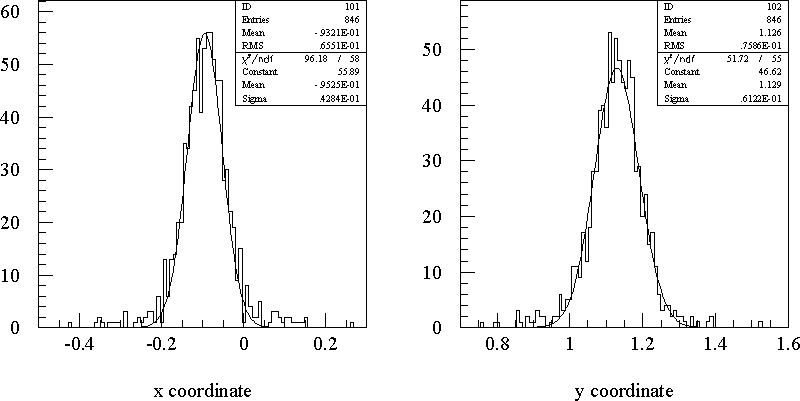
The fact that the method uses one 1 parameter from the data, makes the analysis sensitive to problems in the data itself. In fact, the location of the x-ray collimator is found to be incorrect for many of the runs!The figure linked here shows histograms of the x and y coordinate estimate for a typical run (Run 2508). Fitting the distributions to Gaussians, gives central values of (-0.095 mm,1.129 mm) and standard deviations of 45 and 60 microns in x and y, respectively. These agree well with the assumed collimator position of (-0.100 mm, 1.143 mm). There appears to be little bias in the approach. The data for this run was not used in any way to determine constants for the algorithm. (The only constant is the cloud size, which was determined from the runs with xcol = 0.).
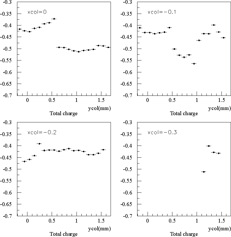
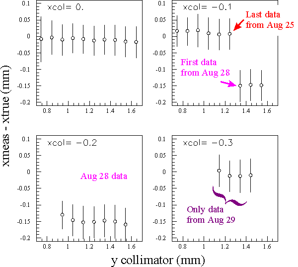
A summary of the x measurement for all runs (where charge sharing can be applied) is shown in the figure linked here. The vertical axis is the difference between the mean estimated and "true" x coordinate of the collimator, and the horizontal axis is the y location of the collimator. The vertical bars represent the standard deviation of the Gaussian fit to the data (ie. the resolution for each event). Something unusual occurred between August 25 and August 28. The data clearly indicates that the x-coordinate of the collimator moved from x = -0.1 mm to x = -0.25 mm. By August 29, the collimator was correctly reset to x= -0.3 mm.
There is no evidence of bias (the collimator - gem positioning is not known to better than about 10 microns, and the August 28 experience shows the the collimator location is not completely stable). The resolution of the x-coordinate is about 45 microns over the entire region where charge sharing can be used.
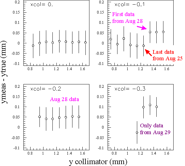
The summary of the y coordinate measurements given in the figure linked here, shows more systematic shifts during the data taking. During the Aug 25 - Aug 28 period, the y-coordinate of the collimator also moved +50 microns. There is also a shift seen during August 29 of about 100 microns in y. In these figures, the vertical bars represent the standard deviation (one event resolution) and not the error in the mean of the 800 events used from each run. The deviations in the residuals have extremely high significance (50 sigma or more!). The deviations during the data taken in Aug 25 (ycol between 0.743 and 0.943) are very significant as well. The resolution of the y-coordinate is about 55 microns over the entire region.
In future runs, the collimator should be brought back to the reference location (3-pad vertex) frequently, to ensure that the location is well understood. [Note: after the analysis was performed, it was noted the signal cable connector was physically re-seated on the detector between the Aug 25 and 28 runs. This was likely responsible for the movement seen in the data. Before the Aug 29 run, the collimator was brought back to the reference location.]
Estimating the number of electrons in the cloud
The figure linked here shows the resolution as a function of the total charge signal. As expected, the resolution is better for events with a large signal. Fits are performed to the simple function: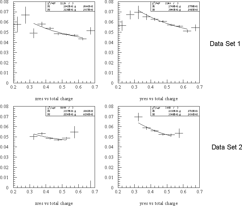
res = sqrt(p12 + p22/Q)where Q is the total charge of the event. The parameter p1 represents the beam size, whereas p2 represents the diffusion term. The x and y resolutions are studied for two different sets of data. The table below gives the results of these simple fits.
The effective number of electrons estimated this way is about a factor two smaller than the number estimated from the knowledge of the x-ray energy and the gas properties. There may be some loss in the primary electron statistics.
sig_beam (microns) < N_electrons> x1 20 +/- 10 70 +/- 10 y1 20 +/- 30 50 +/- 10 x2 35 +/- 10 120 +/- 50 y2 15 +/- 30 50 +/- 10
Summary of charge sharing results
The new method provides an excellent technique for determining the spatial coordinate of the charge cloud centroid. Biases are below the current experimental systematics. The single event resolution is about 50 microns in x and y, about 1/50 of the pitch of the pads. The resolution is not determined by the size of the pads; the algorithm uses only the cloud size (370 microns) to define the scale. Smaller pad sizes would increase the fraction of the area where charge sharing can be used. With the present setup the efficient regions are indicated in the figure linked here. For the study of the capability of position measurements from direct and induced pulses, the pad size is near optimal. Smaller pads would complicate the charge sharing algorithms, and reduce the regions where induced pulses are important.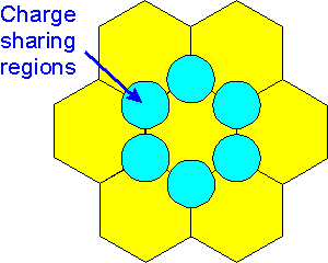
Position analysis from induced pulses
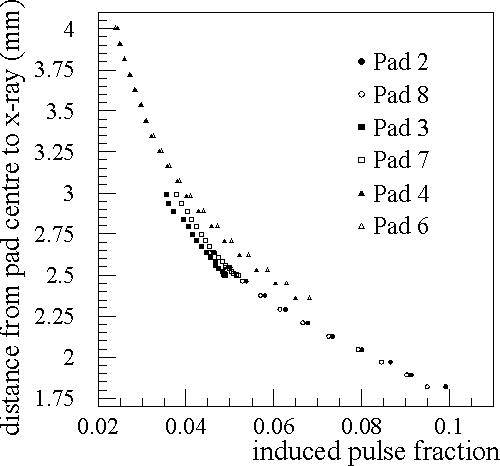
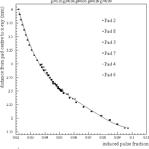
To determine the coordinate from induced pulses, the same approach is used as in the first gem analysis. The amplitude of the induced pulse is assumed to be proportional to the total charge of the event and a function of the distance from the cloud centroid to the pad centre. An algorithm combines the radial information from all pads that have an induced pulse to determine the x-ray location.The data taken along the line (x=0) is used to characterize the induced response function. The ratio of the peak amplitude of the induced pulse to the total charge of the event is shown as a function of distance to the pad centre is shown in the figure linked here. The response function from the various pads do not line up. This is assumed to be due to unequal gains of the preamps, and so scaling factors (up to as much as 10%) are applied to the observed pulse amplitudes (one for each each pad). This improves the agreement, as shown in the figure linked here, so that a universal pad response function can be used. This function defined by a fourth order polynomial fit to the data, shown in the previous figure.
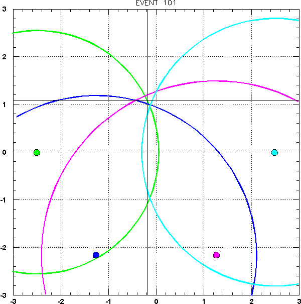
An example of a typical event reconstruction is shown in the figure linked here. The circular arcs represents the deduced distance to the cloud centroid from each of the pads with induced signals. The point which most closely represents the intersection of the circles is shown by the black cross hairs. For this particular run the collimator was located at the coordinate, (-0.100,1.143).
The summary of the x measurements are shown in the figure linked here. The vertical axis is the difference between the measured x location and the "true" location (as defined in the table at the top of this document). The vertical bars represent the standard deviation from fits of the data to Gaussians (single event resolution). Shifts in collimator position found in the charge sharing analysis have not been taken into account, in order to simplify the comparison of the results from the two analyses. The shift in the collimator between August 25 and 28 is confirmed by the induction measurements. Before that time, there is no signifigant bias in the x-coordinate measurement. The data from August 28 shows a strong variation in the bias. This could be caused by unstable gain in one of the induction pads for example. The resolution of x-coordinate measurements from the induction signal is about 50 microns near the centre of the pad (when there are 6 induction measurements) and increases to 80 microns near the edge of the pad.
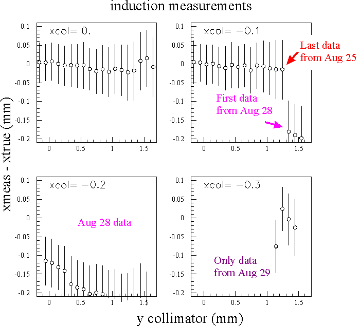
The same figure for the y measurements are shown in the figure linked here. The imperfect matching of the response function for pads 3 and 7 appear to cause biases of order 50 microns. A more careful matching would be able to reduce the bias for the xcol=0 data (and presumably for the other data as well). The resolution of y-coordinate measurements vary from 60 microns near the centre of the pad to 100 microns at the edge.
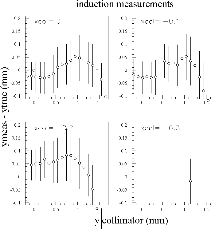
The induction measurements give high precision position measurements in the regions where the charge sharing algorithm does not work. Interestingly, with the present setup, the resolution near the centre of the pad is about the same as the resolution using charge sharing at the edges of the pads. This would be expected if the two measurements are both limited by diffusion.
The induction method is more sensitive to detector systematics. The bias variation from run to run is stronger than in the data from the charge sharing. This is not surprising since the induced signals have a much smaller amplitude. It was shown above that the baseline of the induced pulses appear to move from one run to the next (perhaps due to cross talk between channels). A shift in the baseline by 2 mV of an induced signal, can shift its deduced radius to the beam centroid by 150 microns. Since several pads are used to estimate the position, the overall bias is reduced but still could explain the bias variation that is seen of order 50 microns.
Combination of charge sharing and induced measurements
The figure linked here shows for all 58 runs the residuals for the charge sharing measurements, and for the induced measurements for those events without a charge sharing measurement. The widths are somewhat larger due to uncorrected biases from run to run.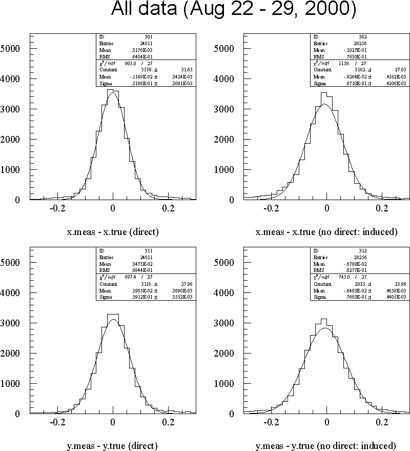
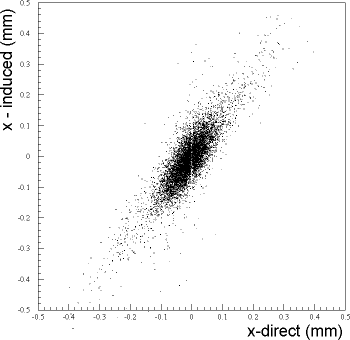
The resolution in the two methods appear to both be limited by diffusion. In that case the two measurements would be highly correlated. This is seen to be the case, and an example is shown in the figure linked here, showing the data at collimator positions at x=0. For events with both charge sharing and induced measurements available, little is gained by combining the two measurements.