Warning: jsMath requires JavaScript to process the mathematics on this page.
If your browser supports JavaScript, be sure it is enabled.

Cosmic Dynamics: Solutions of Friedmann Equations I

Friedmann Equations Solutions

We have

\color{red}{ \left( {\frac{{\dot a}}{a}} \right)^2 = \frac{{8\pi G}}{{3c^2 }}\varepsilon _{} \left( t \right) - \frac{{\kappa c^2 }}{{\left( {R_0 a\left( t \right)} \right)^2 }} + \frac{\Lambda }{3}}

Easy to solve this numerically in general, but we'll solve for some special "one-component universes", mainly flat universes, \color{red}{\kappa = 0}

But the easiest is an empty universe: \color{red}{\kappa = -1}
Matter dominated:
\color{red}{ \kappa = 0,\Lambda = 0,\epsilon _{matter} \ne 0,\epsilon _{radiation} = 0}
Radiation-dominated:
\color{red}{ \kappa = 0,\Lambda = 0,\epsilon _{matter} = 0,\epsilon _{radiation} \ne 0}
"Inflationary type"
\color{red}{ \kappa = 0,\Lambda \ne 0,\epsilon _{matter} = 0,\epsilon _{radiation} = 0}
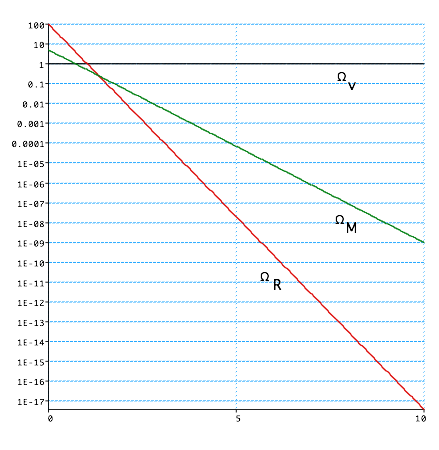
These are independent, but we'll see that any reasonable universe has a dominant term: e.g we can split the universe with matter and radiation into 2 distinct phases: Matter dominated and radiation dominated

The empty universe

May seem silly but is approx correct for a universe with \color{red}{\Omega \ll 1,\Lambda = 0}. Like F = ma with no force!

\color{red}{ \left( {\frac{{\dot a}}{a}} \right)^2 = - \frac{{\kappa c^2 }}{{\left( {R_0 a\left( t \right)} \right)^2 }}}

which is easy:

\color{red}{ \begin{array}{l} {\rm{\dot a = }} \pm \frac{{\rm{c}}}{{{\rm{R}}_{\rm{0}} }} \\ a\left( t \right) = \frac{t}{{t_0 }} \\ \end{array}}

Note we can't have \color{red}{\kappa = +1} since this gives a negative value for \color{red}{{\dot a^2 }} which is unphysical.
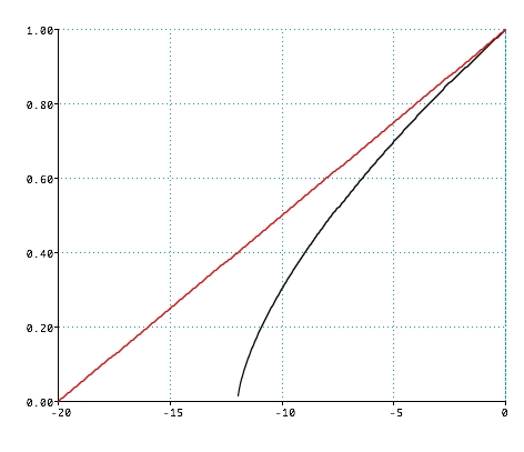
Note that even tho the scale factor increases monotonically, this has non-obvious consequences for distances: galaxy at a redshift z is at a proper distance
\color{red}{ d_p \left( t \right) = c\int_{t_e }^{t_o } {\frac{{dt}}{{a\left( t \right)}}} = ct_o \ln \left( {\frac{{t_o }}{{t_e }}} \right) = \frac{c}{{H_0 }}\ln \left( {1 + z} \right)}

Can now solve easily for flat universe: for matter (radiation)

\color{red}{ \varepsilon _m = \frac{{\varepsilon _{m,0} }}{{a^3 }},\left( {\varepsilon _r = \frac{{\varepsilon _{r,0} }}{{a^4 }}} \right)}

Generically \color{red}{\varepsilon _w = \frac{{\varepsilon _{w,0} }}{{a^{3\left( {1 + w} \right)} }}} so :

\color{red}{ \left( {\frac{{\dot a}}{a}} \right)^2 = \frac{8}{3}\pi G\varepsilon _0 a^n ,n = - 3\left( {1 + w} \right)}

where n = 3 (matter) or 4 (radiation) or anything else (\color{red}{w \ne 1} )

So we want the relation between t and a or ε

\color{red}{\dot a = \sqrt {\frac{{8\pi G\varepsilon _0 }}{{3c^2 }}} a^{ - \frac{{1 + 3w}}{2}} }

The Solution is............

\color{red}{a\left( t \right) = \left( {\frac{t}{{t_0 }}} \right)^{2/(3 + 3w)} ,t_0 = \frac{1}{{1 + w}}\sqrt {\frac{{c^2 }}{{6\pi G\varepsilon _0 }}} }
Hubble's "constant" is $$ \color{red}{ H = \frac{v}{d} = \frac{{\dot a}}{a} = \frac{2}{{nt}}} $$
Note:
For small t, v(t) ≈ 1/R(t) >> c => the horizon problem. No immediate problem with relativity, (since no info is transferred but ...
Parts of the universe have never been in contact with each other.
How do they know to be at the same temperature?
For critical universe Ω=1 as before $$ \color{red}{ \epsilon _c = \rho _c c^2 = \frac{{3H^2 c^2 }}{{8\pi G}}} $$

Expansion time:

\color{red}{a\left( t \right) = \left( {\frac{t}{{t_0 }}} \right)^{2/3} } (t₀ is "now")
Hubbles "constant" in this model

\color{red}{ H\left( {t_{} } \right) = \frac{{\dot a\left( t \right)}}{{a\left( t \right)}} = \frac{2}{{3t}}}

If we take t₀ as the time now since the Big Bang

\color{red}{ t_0 = \frac{2}{3}H^{ - 1} \approx 10^{10} yrs}

(i.e. age of universe is 2/3 of Hubble time)

Matter Only:

Also useful to talk about the Hubble distance: (crudely) most distant thing we could see

\color{red}{ d_H = ct_0 \approx 3.15Gpc}

Density

How does the density change in this model? <

\color{red}{ \rho \left( t \right) = \rho _0 \frac{{a_0^3 }}{{a_{}^3 }} = \frac{{\rho _0 }}{{a\left( t \right)_{}^3 }}}

Note: we are talking about matter density here

Radiation Only

If we have only radiation $$ \color{red}{ \epsilon = \frac{{4\sigma T^4 }}{{c^3 }}} $$

which gives an exact expression for the temp: $$ \color{red}{ T^2 = \frac{1}{t}\sqrt {\frac{{3c^3 }}{{64\pi G\sigma }}} ,t = \frac{\xi }{{T^2 }}} $$

More exactly: from the Black Body equation:

Energy density:

\color{red}{ u = \frac{{8\pi }}{{15}}\frac{{k^4 }}{{h^3 c^3 }}T^4 = \frac{{4\sigma T^4 }}{c}}

(Stef.-Boltz.)
Photon density N ≈ 20 x 10⁶ T³ m^-3

Mean γ-energy E ≈ 2 x 10^-4 T eV

Inflationary Universes

One more special case: how about if vacuum itself has an energy

\color{red}{ \varepsilon _V = \frac{{\Lambda c^2 }}{3}}

Obviously $$ \color{red}{ \frac{{d\rho _v }}{{dt}} = 0} $$

so (setting ρ_m= ρ_r=0 for simplicity) we can use $$ \color{red}{ \left( {\frac{{\dot a}}{a}} \right)^2 = \frac{\Lambda }{3}} $$
which is our previous results with w = -1: this gives$$ \color{red}{ a(t) = a_0 e^{\sqrt {\frac{\Lambda }{3}} t} } $$
i.e. the universe expands exponentially.
Why would we want this?

Energy densities

Three energy densities: \color{red}{\varepsilon _m ,\varepsilon _r ,\varepsilon _\Lambda } give us a total density param

\color{red}{ \Omega = \Omega _m + \Omega _r + \Omega _\Lambda }

Our best bets (Benchmark Model) are

For γ's \color{red}{\varepsilon _\gamma = \alpha T^4 = .26} MeV m^-3
for ν's: 3 varieties, massless, each has \color{red}{\varepsilon _\nu \approx .06} MeV m^-3
for nucleons (baryons), \color{red}{N_B \sim .1} m^-3 \color{red}{ \Rightarrow \varepsilon _B \approx 100} MeV m^-3
for "matter" including dark matter \color{red}{\varepsilon _m \approx 1} GeV m^-3
for vacuum energy, \color{red}{\varepsilon _\Lambda \approx 2} GeV m^-3

or in terms of Ω,

\color{red}{\Omega _r = 10^{ - 4} }
\color{red}{\Omega _m = .3}
\color{red}{\Omega _\Lambda = .7}

(we'll justify all of these later).

Can use this to answer various questions: These have different scaling laws

When did the universe stop being radiation dominated?

Need the R dependence of energy density, ρ

suppose all the matter was Non-Relativistic Matter (e.g. Baryons):

Relativistic particles (i.e. γ's, ν's) get red-shifted as well, so

\color{red}{ \begin{array}{*{20}c} {\varepsilon _m = \frac{{\varepsilon _{m,0} }}{{a^3 }},\varepsilon _{m,0} = 940} \\ {\varepsilon _r = \frac{{\varepsilon _{r,0} }}{{a^4 }},\varepsilon _{r,0} = .26} \\ \end{array}}

We live in matter dominated universe: \color{red}{\varepsilon _M > > \varepsilon _R } , but it was not always thus

So these were equal when:

\color{red}{ a\left( t \right) = \frac{{\varepsilon _{r,0} }}{{\varepsilon _{m,0} }} \approx \frac{1}{{3600}}}

(universe was 1/3600 of current size) or z ≈ 3600

Photon freezeout:

Thermal equilibrium between matter and radiation implies they are at the same mean energy, with a Black Body distribution of γ's. Expansion ⇒ Cooling.

The universe was originally opaque (i.e. mean free path of γ's very small) and hence CMBR was in thermal equilibrium with matter. Then the universe "condensed" (or froze) out.

As the peak in the BB curve falls below hydrogen binding energy, ¹H forms, at ~3700 K, ie about ¹/₂eV. When did this happen?

(Note, this is less than the 13.6 eV that you would expect: need Saha equation)

When was the temp 3700K?.

\color{red}{ t \approx \frac{\zeta }{{T^2 }} \approx 5 \times 10^5 yrs}

or z ≈1360: i.e, at about the same time that the universe became matter-dominated. (Note: we began with a very large uncertainty, setting Ω ≈ 0.01, based on .03 proton per cubic metre: depending on the nature of the DM we can change this by a factor of 10)

we'll improve both these numbers a bit with more realistic universes later

Multi Component Solutions

We have

\color{red}{ \left( {\frac{{\dot a\left( t \right)}}{{a\left( t \right)}}} \right)^2 = \frac{{8\pi G}}{{3c^2 }}\varepsilon \left( t \right) - \frac{{\kappa c^2 }}{{R_0^2 a\left( t \right)^2 }} + \frac{\Lambda }{3}}

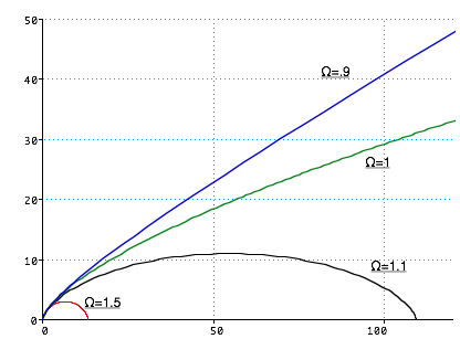
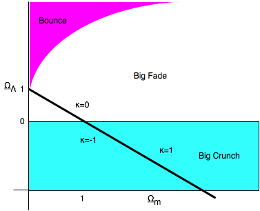
More realistic univerese are going to have 2-4 components. We'll follow Ryden in using Ω as the energy variable of choice: Ω_k,0 is the current value of the k'th density param: or in terms of Ω,

Radiation (Massless particles) \color{red}{\Omega _{r,0} = 10^{ - 4} }
Matter (Massive Particles)\color{red}{\Omega _{m,0} }
Cosmological Constant \color{red}{\Omega _{\Lambda ,0} }
Total \color{red}{\Omega _{0} }

lump Λ into the energy.

Can eliminate κ in favour of Ω₀:

\color{red}{ H\left( t \right)^2 = \frac{{8\pi G}}{{3c^2 }}\varepsilon \left( t \right) - \frac{{H_0^2 }}{{a\left( t \right)^2 }}\left( {\Omega _0 - 1} \right)}

\color{red}{ \frac{{H\left( t \right)^2 }}{{H_0^2 }} = \frac{{\varepsilon \left( t \right)}}{{\varepsilon _{c,0} }} + \frac{{\left( {1 - \Omega _0 } \right)}}{{a\left( t \right)^2 }}}

(Note \color{red}{\left( {\Omega _0 - 1} \right)}: will see that the nature of solution changes drastically if this is + or -).

Putting in the correct scaling laws, this gives us the general solution

\color{red}{ H_0^{} t = \int_{}^{} {\frac{{da}}{{\sqrt {\frac{{\Omega _{r,0} }}{{a^2 }} + \frac{{\Omega _{m,0} }}{a} + \Omega _{\Lambda ,0} a^2 + \left( {1 - \Omega _0 } \right)} }}} }

Not ideal: we'd like a(t), not t(a), and we can't do the general case explicitly

Matter-Curvature

SImple equation

\color{red}{ \frac{{H\left( t \right)^2 }}{{H_0^2 }} = \frac{{\Omega _0 }}{{a^3 }} + \frac{{\left( {1 - \Omega _0 } \right)}}{{a\left( t \right)^2 }}}

Note H₀ > 0, so universe will

always expand ( H(t) > 0) if Ω₀ < 1: (Big Fade)
stop asymptotically ( H(t) ⇒ 0) if Ω₀ = 1:
expand to max and contract if if Ω₀ > 1: (Big Crunch)

Just a restating of the non-rel model we had earlier.

Parametric solution

\color{red}{ \begin{array}{l} a\left( \theta \right) = \frac{{\Omega _0 }}{{2\left( {\Omega _0 - 1} \right)}}\left( {1 - \cos \left( \theta \right)} \right) \\ t\left( \theta \right) = \frac{1}{{2H_0 }}\frac{{\Omega _0 }}{{\left( {\Omega _0 - 1} \right)^{3/2} }}\left( {\theta - \sin \left( \theta \right)} \right) \\ \end{array}}

for Ω₀ > 1: etc.

Oh I've seen fire and I've seen rain

I've seen sunny days that I thought would never end

James Taylor

Lifetime of universe in Big Crunch models is given by
\color{red}{ t_c = \frac{{\Omega _0 \pi }}{{H_0 \left( {\Omega _0 - 1} \right)^{3/2} }}}
Note for small t (small θ) these all expand at as a(t) ∼ t^2/3

Matter-Lambda

Will assume that we are at critical density, so

\color{red}{ \Omega _0 = 1 = \Omega _{m,0} + \Omega _{\Lambda ,0} }

SImple equation again

\color{red}{ \frac{{H\left( t \right)^2 }}{{H_0^2 }} = \frac{{\Omega _{m,0} }}{{a^3 }} + \left( {1 - \Omega _{m,0} } \right)}

Again note importance of \color{red}{\left( {\Omega _{m,0} - 1} \right)}: will see that the nature of solution changes drastically if this is + or -).

Explicit solution possible:

\color{red}{ \begin{array}{l} a\left( t \right) = \sqrt {\frac{{\Omega _{m,0} }}{{\Omega _{m,0} - 1}}} \left( {\sin \left( {\frac{3}{2}\left( {\Omega _{m,0} - 1} \right)t} \right)} \right)^{2/3} \Omega _{m,0} > 1 \\ a\left( t \right) = \sqrt {\frac{{\Omega _{m,0} }}{{1 - \Omega _{m,0} }}} \left( {\sinh \left( {\frac{3}{2}\left( {1 - \Omega _{m,0} } \right)t} \right)} \right)^{2/3} \Omega _{m,0} < 1 \\ \end{array}}

Note we get

Runaway solution if Ω_m,0 < 1, which implies Ω_Λ,0 > 0,
Big crunch solution if Ω_m,0 > 1, which implies Ω_Λ,0 < 0,
Our best bets (Benchmark Model) has
- \color{red}{\Omega _r = 10^{ - 4} }
- \color{red}{\Omega _m = .3}
- \color{red}{\Omega _\Lambda = .7}
This gives \color{red}{\Omega _m = \Omega _\Lambda } at about 10¹⁰ years: i.e. we are now in and expanding phase

Matter-Curvature-Lambda

\color{red}{ \frac{{H\left( t \right)^2 }}{{H_0^2 }} = \frac{{\Omega _{m,0} }}{{a^3 }} + \frac{{\left( {1 - \Omega _{m,0} - \Omega _{\Lambda ,0} } \right)}}{{a^2 }} + \Omega _{\Lambda ,0} }

By adjusting (fiddling) parameters we can get the following generic behavioiurs

Big Crunch
Big Fade (exponentially expanding )
Big Fade (critical matter universe)
Big Bounce (contracting phase, followed by exponentially expanding phase: note this implies no Big Bang!)
Loitering (adjust Ω_m,0 so that universe almost cruunches but then Ω_Λ,0 > 0 starts winning.

Radiation + Matter

How about radiation? Because of scaling, any universe with a Big Bang is initially dominated by radiation, so can reasonably ignore κ and Ω_Λ so

\color{red}{ \frac{{H\left( t \right)^2 }}{{H_0^2 }} = \frac{{\Omega _{m,0} }}{{a^3 }} + \frac{{\Omega _{r,0} }}{{a^4 }}}

exactly soluble in terms of

\color{red}{ a_{rm} = \frac{{\Omega _{r,0} }}{{\Omega _{m,0} }}}

value of scale factor when matter-density =radn. density up until then, can ignore matter:

\color{red}{ a\left( t \right) = \left( {2\sqrt {\Omega _{r,0} } H_0^{} t} \right)^{1/2} }

Time, distance and red-shift

All very well, but we cannot observe a(t) : how does it relate to red-shift?

Connection between time, distance and red-shift:

At time t₀, a galaxy is at a distance d₀ from us, and is travelling at v

We see the photon at time t₁

In time t between γ emission & absorption, the distance has increased (universe has expanded) by zct. so γ has to travel further: travel time \color{red}{t = \frac{{d_1 }}{c}}
so \color{red}{d_1 = d_0 + zct}
so that \color{red}{d_1 = \frac{{d_0 }}{{1 - z}}}
i.e. if z = .25, the universe was 75% of current size when γ was emitted

(Note we have made a subtle change in the description: it is not the other galaxy which is moving away, it is the space in between which is stretching!)

We can also relate red-shift and age: At t = 0, universe had no size so \color{red}{d_0 = vt_o = zct_0 } hence \color{red}{\frac{{t_0 }}{{t_1 }} = \frac{{d_0 }}{{d_1 }} = 1 - z}
so that \color{red}{t_0 = \left( {1 - z} \right)t_1 }
so again if z = .25, the universe was only 75% of its current age
(Correctly \color{red}{d_1 = d_0 \left( {1 + z} \right)} and \color{red}{t_0 = \frac{{t_1 }}{{1 + z}}} , because of relativistic effects, but we also need to allow for slowing down of the expansion)
Note: the red-shift is more fundamental than the velocities: e.g. we'll talk about z = 3000 for the CMBR, which describes the time at which it was emitted, but it's not really sensible to turn this into v.

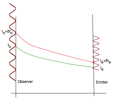
Now we'll do the red-shift calculation properly

Emitting galaxy produces photon, with gap \color{red}{\delta t_e } between crests, observing galaxy sees gap of \color{red}{\delta t_o }

Both crests travel at speed of light so follow null-geodesic

\color{red}{ d\tau ^2 = dt^2 - \frac{{R\left( t \right)^2 }}{{c^2 }}\left( {\frac{{d\sigma ^2 }}{{\left( {1 - \kappa \sigma ^2 } \right)}} + \sigma ^2 d\Omega ^2 } \right) = 0}

We are using Berry notation: so \color{red}{ R(t) = R_0^{} a\left( t \right)} and \color{red}{ \sigma = \frac{x}{{R_0^{} }}} and

\color{red}{ ds^2 = - c^2 dt^2 + a\left( t \right)^2 \left( {\frac{{dx^2 }}{{\left( {1 - \kappa \frac{{x^2 }}{{R_0^2 }}} \right)}} + x^2 d\Omega ^2 } \right)}

so for the first crest
\color{red}{ \int_{t_e }^{t_o } {\frac{{dt}}{{R\left( t \right)}}} = \frac{1}{c}\int_0^{\sigma _e } {\frac{{d\sigma }}{{\sqrt {1 - \kappa \sigma ^2 } }}} }
and for the second,
\color{red}{ \int_{t_e + \delta t_e }^{t_o + \delta t_o } {\frac{{dt}}{{R\left( t \right)}}} = \frac{1}{c}\int_0^{\sigma _e } {\frac{{d\sigma }}{{\sqrt {1 - \kappa \sigma ^2 } }}} }

so that

\color{red}{ \int_{t_e }^{t_o } {\frac{{dt}}{{R\left( t \right)}}} = \int_{t_e + \delta t_e }^{t_o + \delta t_o } {\frac{{dt}}{{R\left( t \right)}}} }
\color{red}{ \begin{array}{l} \int_{t_e + \delta t_e }^{t_o + \delta t_o } {\frac{{dt}}{{R\left( t \right)}}} = \int_{t_e }^{t_o } {\frac{{dt}}{{R\left( t \right)}}} - \int_{t_e }^{t_e + \delta t_e } {\frac{{dt}}{{R\left( t \right)}} + } \int_{t_o }^{t_o + \delta t_o } {\frac{{dt}}{{R\left( t \right)}}} \\ \Rightarrow \frac{{\delta t_o }}{{R\left( {t_o } \right)}} - \frac{{\delta t_e }}{{R\left( {t_e } \right)}} = 0 \\ \end{array}}
Expanding this (valid since times are short)
\color{red}{ \frac{{\lambda _o }}{{\lambda _e }} = \frac{{c\delta t_o }}{{c\delta t_e }} = \frac{{R\left( {t_o } \right)}}{{R\left( {t_e } \right)}}= \frac{{a\left( {t_o } \right)}}{{a\left( {t_e } \right)}}}
Note normally this will happen: the dimensional quantities will cancel
Hence Red-shift $\color{red}{z = \frac{{a\left( {t_o } \right)}}{{a\left( {t_e } \right)}} - 1}$ is given the ratio of the size of the universe when it was emitted to now (obviously!). We can then expand this
\color{red}{ a\left( {t_e } \right) = a\left( {t_o } \right) + \left( {t_e - t_o } \right)\dot a\left( {t_o } \right) + \frac{1}{2}\left( {t_e - t_o } \right)^2 \ddot a\left( {t_o } \right) + .....}
assumes the universe has been expanding smoothly over the time interval between emission and observation.

so that

Can then use the present value of the Hubble param.
\color{red}{ H_0 = H\left( {t_o } \right) = \frac{{\dot a\left( {t_o } \right)}}{{a\left( {t_o } \right)}}}
\color{red}{ a\left( {t_e } \right) = a\left( {t_o } \right)\left( {1 + \left( {t_e - t_o } \right)H_0 - \frac{1}{2}\left( {t_e - t_o } \right)^2 H_0 ^2 q_0 + .....} \right)}
where
\color{red}{ q_0 = - \frac{{\ddot a\left( {t_o } \right)a\left( {t_o } \right)}}{{\dot a\left( {t_o } \right)^2 }} = - \frac{{\ddot a\left( {t_o } \right)}}{{a\left( {t_o } \right)H_0 ^2 }}}
Deceleration Parameter defined in this odd way so that q₀ =1 if the universe is a critical one.
What is q₀ if universe is empty?

Other Observables

In similar ways, we get

Hubble plot corrections $\color{red}{z = H_0 \left( {t_0 - t_E } \right) + \left( {1 + \frac{1}{2}q_0 } \right)\left( {t_0 - t_E } \right)^2 + .....}$
Object horizon (distance of most distant object we can see now
$\color{red}{\int_{t_{\min } }^{t_o } {\frac{{dt}}{{R\left( t \right)}}} = \int_0^{r '} {\frac{{dr }}{{\sqrt {1 - \kappa \sigma ^2 }}}} }$ (note that in some $\kappa =1$ models we can see the whole universe!)
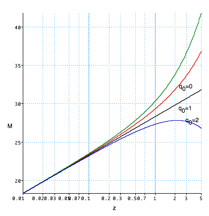
Apparent luminosity: $\color{red}{l = \frac{L}{{4\pi D^2 }} \Rightarrow l = \frac{L}{{4\pi a\left( t \right)^2 r _E^2 }}}$:
again can expand result to give $\color{red}{l = \frac{{LH_0 ^2 }}{{4\pi c^2 z_{}^2 }}\left[ {1 + \left( {q_0 - 1} \right)z + ...} \right]}$

Since we measure magnitudes, better to use
$\color{red}{m - M \approx 25 - 5\log H_0 + 5\log \left( {cz} \right) + \left( {1 - q_0 } \right)z}$

Hence importance of 1a supernovae: since we know (maybe) L, we can get $q_0$ directly.
- Olber's paradox: total luminosity will depend on density of galaxies [n(t)] as well as luminosity of each
  $\color{red}{l_{tot} = \frac{{cn\left( {t_o } \right)}}{{a\left( {t_o } \right)}}\int_{t_{\min } }^{t_o } {L\left( t \right)a\left( t \right)dt} }$
  so it will be finite for t_min = 0 (i.e. models with a Big Bang) but allows us to rule out other models
Number counts: How can we decide if universe is closed or open? This becomes an observational question: density of galaxies at different distances depends on $\kappa$
- Note that all have same density of galaxies but (e.g.) $\kappa = 1$ has fewer galaxies at large distances
  (Earth has less land at large distance than a flat plane would have!)
- Observationally this could be done via Hubble plot at very large distance:
  Unfortunately, only individual objects that can be seen at these red-shifts are quasars: these have evolved since the BB and hence cannot be used as constant density markers
  Since the density of matter is so important, we'll look at that now