Index

• Gem pad layout
• Gem data
• Gem data analysis programs
• Separation of direct and induced components of signals
• Gain variation
• Pedestals
• Position analysis from direct charge sharing
• Observed charge fraction in pad 1 - determination of cloud size
• Determining position from charge fractions
• Position analysis from induced pulses
• Calibration data part 1
• Calibration data part 2
• Conclusion

GEM pad layout

GEM data

The 60 data runs are summarized below. The collimator location is indicated using the coordinate system described above. The first two digits of the run number is the day of the month that the data was taken.

Before the run 2403, the xay collimator was brought back to the vertex position. A realignment was necessary at that time to bring the signal sizes on the 3 pads to agreement. The x and y position of the collimator was shifted in the negative direction by 30 microns. Unfortunately, pad-pad gain measurements were not made. The GEM system failed after the runs recorded here, requiring the GEM box to be opened for investigation of the problem.

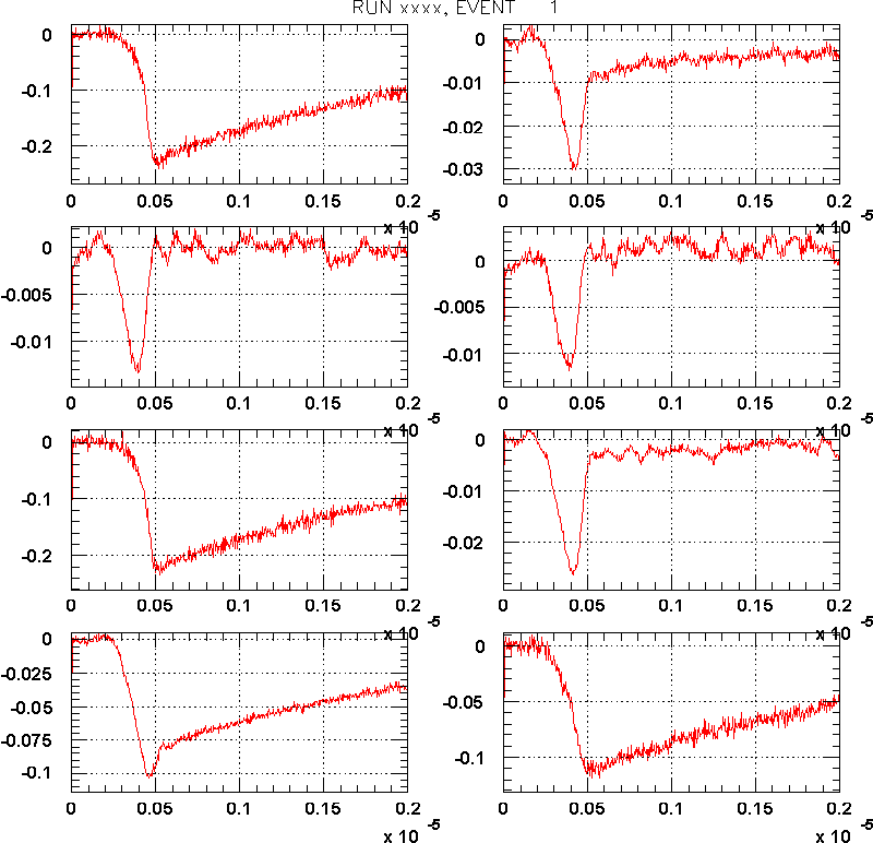
As an example, the first event from run 2201 is shown here.

run number x_coll (mm) y_coll (mm) 2001 0. 1.443 2002 0. 1.043 2003 0. 0.843 2004 0. 0.643 2005 0. 0.443 2006 0. 0.243 2007 0. 0.043 2008 0. -0.157 2009 0.200 -0.157 2010 0.200 0.043 2011 0.200 0.243 2012 0.200 0.443 2013 0.200 0.643 2014 0.200 0.843 2015 0.200 1.043

run number x_coll (mm) y_coll (mm) 2101 0.200 1.243 2102 0.200 1.443 2103 0. 1.443 2104 0. 1.643 2105 0. 1.243 2106 0.400 1.243 2107 0.400 1.043 2108 0.400 0.843 2109 0.400 0.643 2110 0.400 0.443 2111 0.400 0.243 2112 0.400 0.043 2113 0.400 -0.157 2114 0.600 -0.157 2115 0.600 0.043 2116 0.600 0.243 2117 0.600 0.443 2118 0.600 0.643

run number x_coll (mm) y_coll (mm) 2201 0.600 0.843 2202 0.600 1.043 2203 0.800 0.843 2204 0.800 0.643 2205 0.800 0.443 2206 0.800 0.243 2207 0.800 0.043 2208 0.800 -0.157 2209 1.000 -0.157 2210 1.000 0.043

run number x_coll (mm) y_coll (mm) 2301 1.000 0.243 2302 1.000 0.443 2303 1.000 0.643 2304 1.200 0.443 2305 1.200 0.243 2306 1.200 0.043 2307 1.200 -0.157 2308 1.400 -0.157 2309 1.400 0.043 2310 1.400 0.243 2311 1.600 0.043

run number x_coll (mm) y_coll (mm) 2401 1.600 -0.157 2402 1.800 -0.157 2403 0.0 1.443 2404 0.0 1.243 2405 0.0 1.043 2406 0.0 0.843

GEM data analysis programs

Separation of direct and induced components of signals

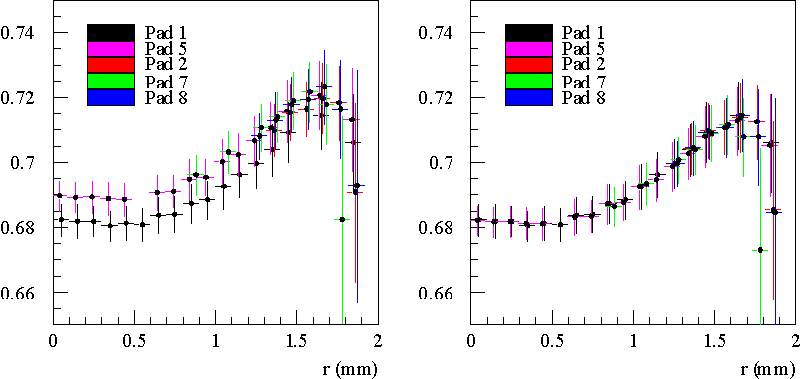
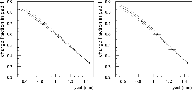
The left plot from the figure linked here shows the mean ratio of the "late" to the peak amplitudes on pads 1,2, 7 and 8 as a function of the distance from the centre of the pad to the collimator position. The error bars indicate the standard deviations of the ratio. (The mean and standard deviations are found by fitting each ratio distribution to a Gaussian). The standard deviation is less than 1%; so the late amplitude is used instead of the peak amplitude for the charge fraction determination of both direct and mixed signals.

The ratio for pad 1 is independent of the location of the xray collimator provided all of the charge is collected by the pad. Surprisingly this ratio initially increases as the xray collimator gets beyond 0.7 mm from the pad centre. The scaling factor for the "late" amplitude for pad 1 is taken to be 0.681 from this data. For the other channels the scaling factor is somewhat larger. The right plot from the figure linked here shows the ratios after a multiplicative correction is applied to bring the channels into better agreement. The reason that channel 1 is different from the rest may be due to the fact that the scope is terminated with 1 MOhm for that channel (because the signal is shared with channel 5) whereas the rest of the channels are terminated with 50 Ohm.

The scaling factors deduced for channels 1,2,5,7,8 are 0.681, 0.686, 0.689, 0.691, 0.689 respectively.

Gain variation

Pedestals

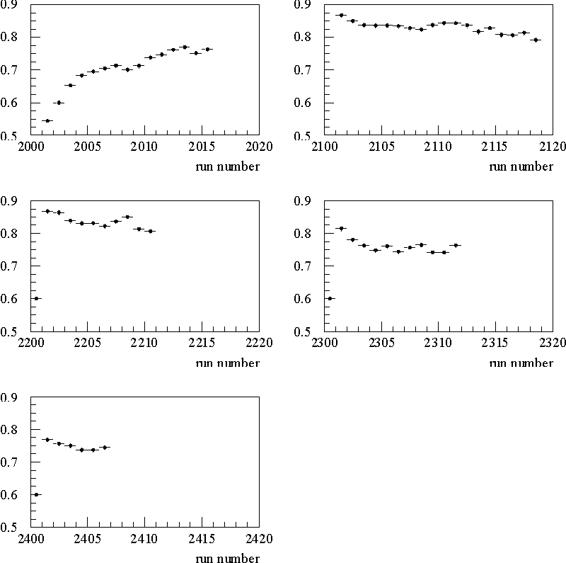
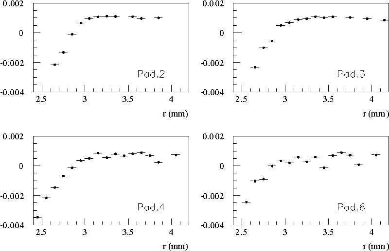
Some plots have been produced to check if the baseline changes from run to run: The pulse shape is fit to a quadratic 300ns - 900 ns after the induced pulse. The value of the fit at the point 600 ns after the pulse defines the "baseline". The value of the baseline for the different runs are shown in the figure linked here. The baseline is seen to be independent of position of the x-ray collimator as long as it is more than about 3.1 mm from the centre of the pad for the for pads, 2,3,4, and 6. The other pads do not have measurements with the x-ray collimator far enough away. There is no evidence for cross talk, which in the past showed up as a dependence of the baseline from one channel on the amplitude of the pulse on another channel.

Position analysis from direct charge sharing

Observed charge fraction in pad 1 - determination of cloud size

Determining position from charge fractions

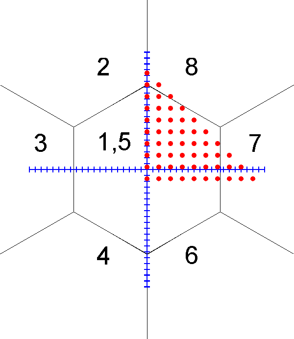
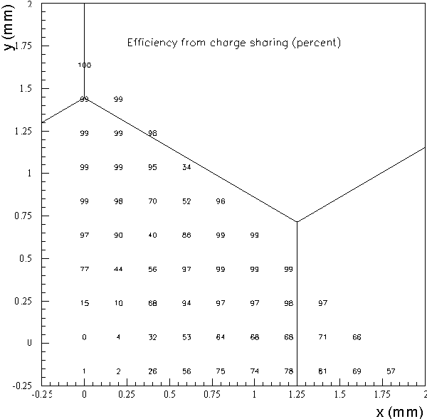
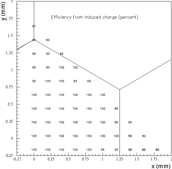
The efficiency for events to have its position determined in this way is summarized in the plot linked here. The lines indicate the pad boundaries and the efficiencies are printed at the micrometer readings of the x-ray collimator. Low efficiency is found in regions where the charge is shared amongst fewer or more than 3 pads. Some inefficiency would be recovered by considering events with 4 pads that share the charge.

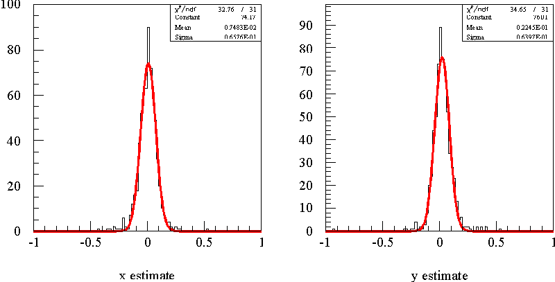
The figure linked here shows histograms of the x and y coordinate estimates, with respect to the x and y collimator position, for run 2106. Fitting the distributions to Gaussians, gives central values of (0.007 mm,0.022 mm) and standard deviations of 66 and 64 microns in x and y, respectively.

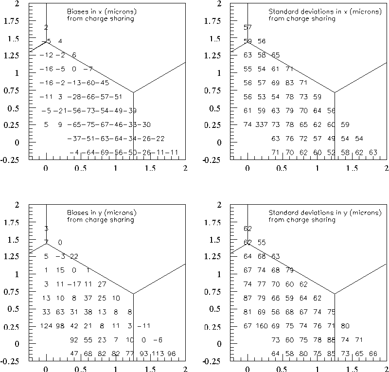
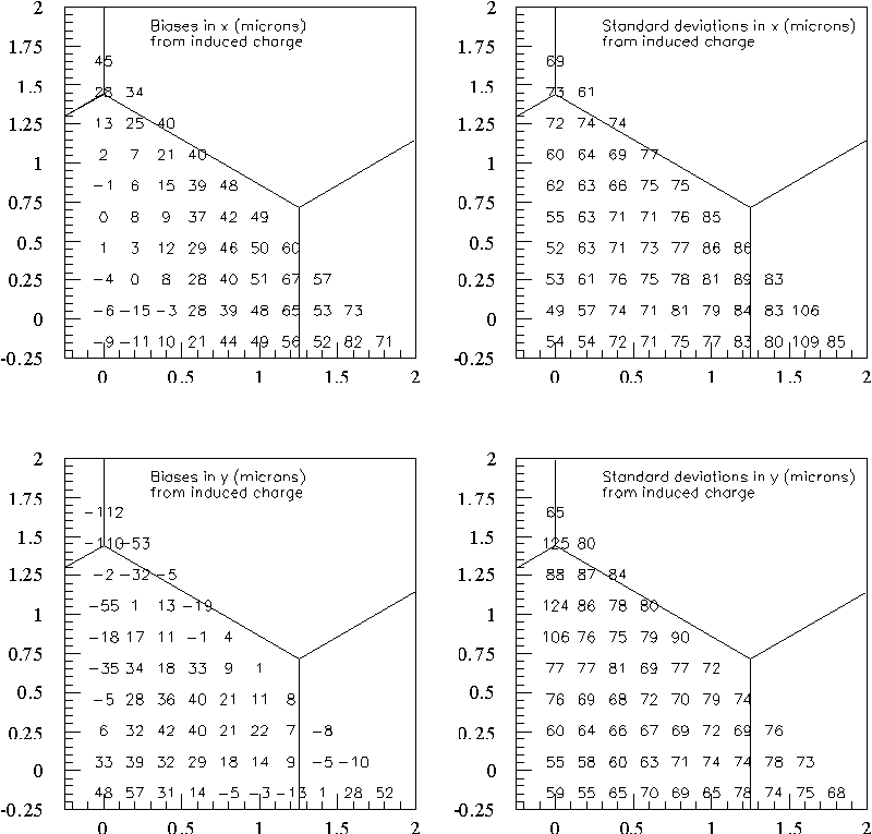
There are regions where the biases in x and y for this measurement are large, as shown in the figures linked here. The standard deviations of the measurements are between 50 and 80 microns throughout the region. The observed biases can result from gain inequalities from pad to pad. It appears, for example, that the gain in pad 7 is smaller than for other pads, resulting in biases towards -x in regions where pad 7 is used to estimate the position.

In the section on position analysis from induced pulses below, the relative gains of the outer 6 pads is deduced by matching their induced pulse height functions. Unfortunately, this does not tie the gain relative to the central pad, leaving that parameter to be determined. That analysis does not support the hypothesis that pad 7 has a smaller gain than pad 2 and 8. The calibration data analysis, however, does support the hypothesis that pad 7 has a smaller gain than pads 2 and 8.

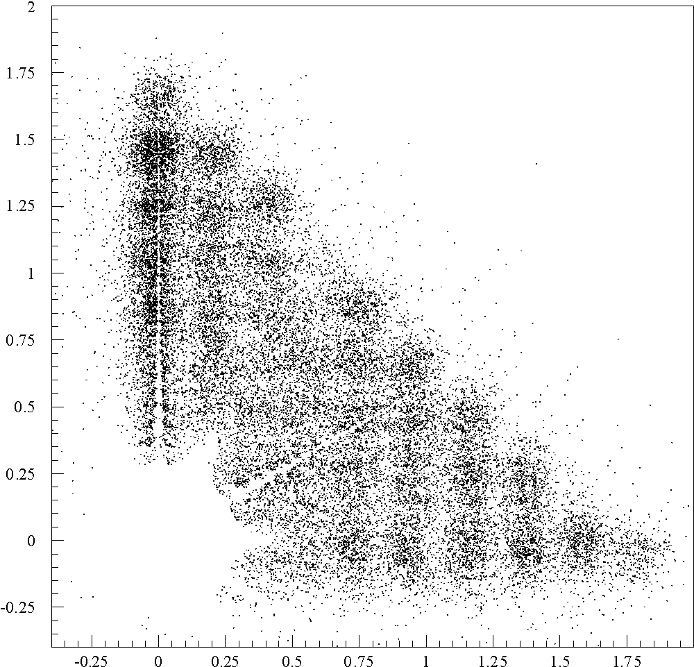
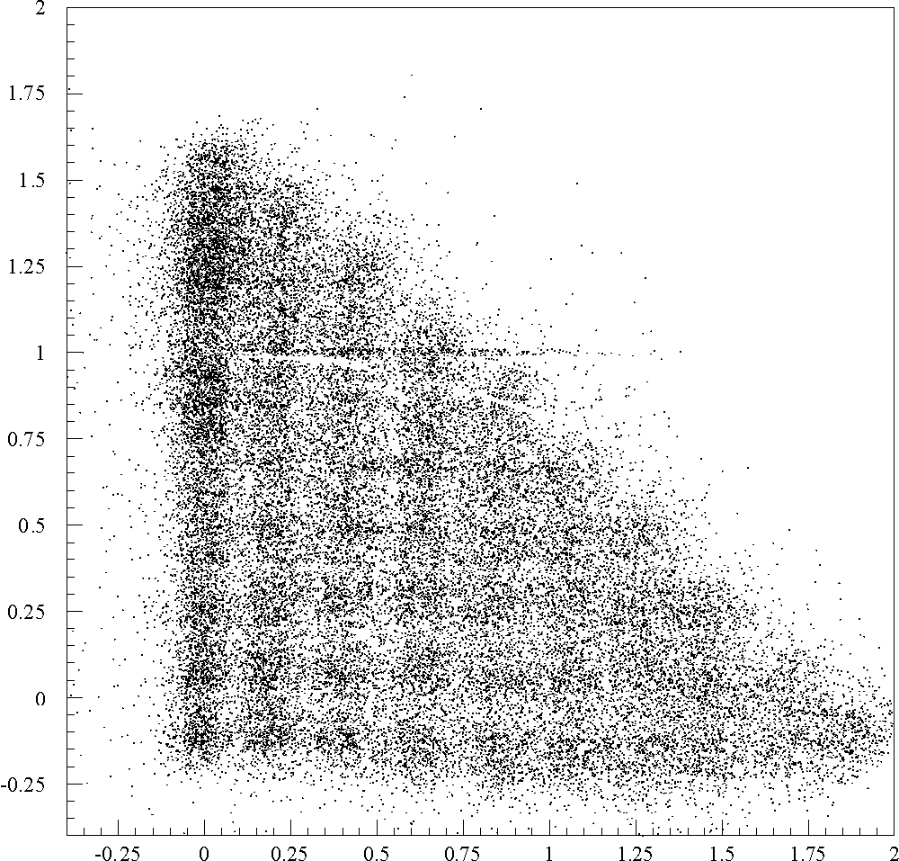
A map of all reconstructed events appears in the figure linked here. The gaps at 30 degrees and 90 degrees are due to a problem with the process of inverting the mapping between cloud centroid and pad charge fractions.

Position analysis from induced pulses

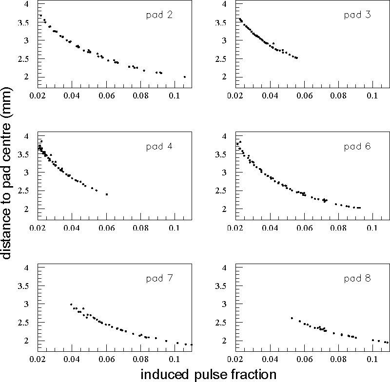
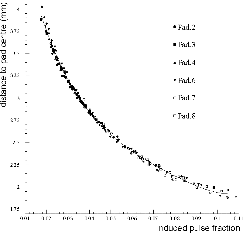
The ratio of the peak amplitude of the induced pulse to the total charge of the event as a function of distance to the pad centre is shown in the figure linked here. Some of the scatter seen for the pads (for example pad 7) is reduced if the first 9 runs and the last 6 runs are ignored. The response functions are overlayed for all the pads in the figure linked here. In order to match the curves, the signals in pads 2, 7, and 8 were scaled by factors 0.93, 0.95, and 0.95 respectively. The curve is the result of a fit to a 4th order polynomial that is used in the analysis to describe the response function.

The efficiency for events to have the x-ray position successfully determined with the induced pulse method is quite high, as summarized in the figure linked here. The bias and standard deviations of the measurements are shown in the figure linked here. The region centered on pad 1, but near pad 7 has a bias in the +x direction, whereas in the direct charge analysis a bias was seen in the opposite direction.

A map of all reconstructed events from induced pulses appears in the figure linked here. An unusual artifact appears near y=1. The grid nature of the data taking is evident.
 

Calibration Data - Part 1

The "late amplitude" is defined as 1200 ns after the peak pulse. The values R1 and R5 are the ratios of the late amplitude to the peak amplitude for channels 1 and 5 (both connected to the centre pad). The values are within about a percent of each other. The average signal (which includes the corrections R1,R5) shows much larger variation, over 10%. The variation could arise from the following sources: (1) changes in operating conditions - gas mixture and charging of GEM; (2) variation in the pre-amplifier gain from channel to channel; and (3) variation in the GEM amplification as a function of position over the GEM.

The mean signal values in the table above were used to define scale factors for the direct charge signals from the November data, and the position analysis from charge sharing was repeated. The relative scale factor for pad 1 could not be determined from the calibration data. A few values were considered, and a value corresponding to mean signal size of 0.71 was selected, as it gave the smallest variance of the position residuals. The average cloud size was also varied to reduce the variance of the position residuals, and the best value was found to be 0.55 mm, instead of the value 0.58 mm that was used above. An offset of (-6,26) microns (x,y) is also applied to bring the central values of the residuals to zero.

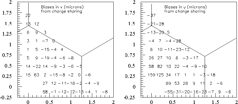
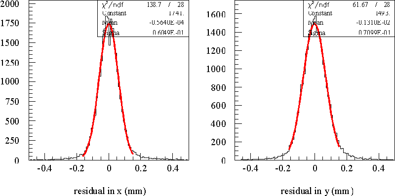
The calibrations described above reduce the scatter in the biases seen across the GEM pad, as shown in the figure linked here. The distributions of residuals for the entire data set is shown in the figure linked here, with the standard deviations in x and y found to be about 60 and 70 microns respectively. A more careful calibration procedure could possibly reduce the biases further. It should be kept in mind that after moving the micrometer stage and returning to its origin there are shifts of order 20 microns observed.
 

Calibration Data - Part 2

The second and last calibration run shows an increase in gain by 4%. The assumed pad 1 gain is taken to increase linearly during the calibration runs, with the value shown in the column labelled "pad1".  Pad 6 is again seen to have the lowest gain. However, the two sets of calibrations show greater variance in the relative mean signals than would be expected from the errors in the means. Comparing the pads that were measured for both sets of runs:
 
 

The gain variation from pad to pad is not reproducible between the two sets of calibration runs. Further studies of the gain stability of the gem would be useful. By taking the second set of pad to pad gain corrections, the overall residual deviations from charge sharing (61,73) microns (x,y) is achieved when the cloud size is reduced to 0.52 mm. The width of the residuals is not quite as good as was found for the previous set of calibration constants. An offset of (25,-33) microns is applied to bring the residuals to a mean of zero.

The induced pulse analysis is repeated using these calibrations as the starting point. No improvement in residual widths is observed.

Conclusion