next up previous
Next: About this document ... Up: tsigex Previous: Conclusion

Bibliography

1
A. Bellerive, Joint PDFs with Projections and Correlations, SNO Note.
manhattan.sno.laurentian.ca/sno/ananoteb.nsf/URL/MANN-5NLT9C.

2
D. Karlen, Using Projections and Correlations to Approximate Probability Distributions, Computers in Physics, 12:4 (1998) 380.

3
G. Cowan, Statistical Data Analysis, Oxford University Press 1998.

4
S. Brandt, Data Analysis, Springer-Verlag 1998.

5
www.physics.carleton.ca/research/sno/anal/software/qsigex.html.

6
Pierre-Luc Drouin and Alain Bellerive, QSigEx 3.1 Manual, SNO Note. manhattan.sno.laurentian.ca/sno/ananoteb.nsf/URL/MANN-5YJRA9.

7
D. Grant, Ph.D. Thesis.

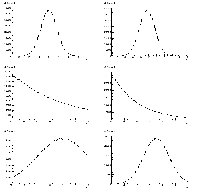
Figure 1: Template of the marginal distributions used for the ensemble test. The random variables $x_1$ and $x_2$ for classes $\ensuremath {{\cal {C}}}_1$, $\ensuremath {{\cal {C}}}_2$, and $\ensuremath {{\cal {C}}}_3$ are shown.
\begin{figure}\centerline{\epsfig{figure=draw_marginal.eps,height=6.5in}}\end{figure}

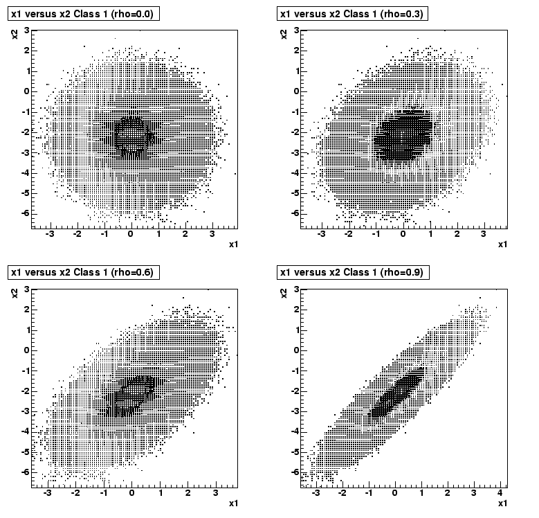
Figure 2: Template of the scatter distribution $x_1$ versus $x_2$ for the class $\ensuremath {{\cal {C}}}_1$ used for the ensemble test. The correlation between the random variables are $\rho _{12}(\ensuremath {{\cal {C}}}_1)=0.0$, $\rho _{12}(\ensuremath {{\cal {C}}}_1)=0.3$, $\rho _{12}(\ensuremath {{\cal {C}}}_1)=0.6$, and $\rho _{12}(\ensuremath {{\cal {C}}}_1)=0.9$.
\begin{figure}\centerline{\epsfig{figure=draw_2d.eps,height=6.5in}}\end{figure}

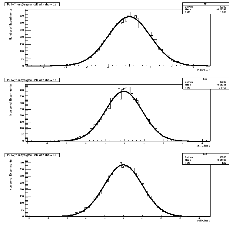
Figure 3: The results of the pull experiment for the multi-D method with $\rho _{12}(\ensuremath {{\cal {C}}}_1)=0.3$. For each experiments we perform the fit for the unknown fraction $\vec{\theta}$ and compute $\ensuremath {{\cal {P}}}= \Delta / \sigma _{\theta _i}$. The value of $\ensuremath {{\cal {P}}}$ is then filled in the histogram for a total entry of 10,000 experiments. Then we compute the mean $\bar{\ensuremath {{\cal{P}}}}=$-0.021, -0.053, and -0.014 for the classes $\ensuremath {{\cal {C}}}_1$, $\ensuremath {{\cal {C}}}_2$, and $\ensuremath {{\cal {C}}}_3$, respectively; and the standard deviation $\sigma _\ensuremath {{\cal {P}}}=$ 1.009, 0.973, and 1.020.
\begin{figure}\centerline{\epsfig{figure=ex_2d_0.3_draw.eps,height=6.5in}}\end{figure}


Table: Results of the ensemble test for the standard method (1D) as a function of the correlation parameter $\rho_{12}(\ensuremath {{\cal{C}}}_1)$. The pull is defined as $\ensuremath {{\cal {P}}}= \Delta / \sigma _{\theta _i}$, where $\Delta = \theta_i({\rm{FIT}})-\theta_i({\rm{MC}})$. The central limit theorem insures that the expectation for $\bar{\ensuremath {{\cal{P}}}}$ is $E(\bar{\ensuremath {{\cal{P}}}})=0$ and the expectation for $\sigma_{\ensuremath {{\cal{P}}}}$ is $E(\sigma_{\ensuremath {{\cal{P}}}})=1$.
Class Method $\rho_{12}(\ensuremath {{\cal{C}}}_1)$ Mean $\bar{\ensuremath {{\cal{P}}}}$ Sigma $\sigma_{\ensuremath {{\cal{P}}}}$
C1 1D 0.0 -0.0198238 $\pm$ 0.010 1.006 $\pm$ 0.007
C2 1D 0.0 -0.0485768 $\pm$ 0.010 0.971 $\pm$ 0.007
C3 1D 0.0 -0.0201215 $\pm$ 0.010 1.021 $\pm$ 0.007
C1 1D 0.1 -0.0481886 $\pm$ 0.010 1.007 $\pm$ 0.007
C2 1D 0.1 -0.0579881 $\pm$ 0.010 0.972 $\pm$ 0.007
C3 1D 0.1 0.0174762 $\pm$ 0.010 1.020 $\pm$ 0.007
C1 1D 0.2 -0.0709891 $\pm$ 0.010 1.007 $\pm$ 0.007
C2 1D 0.2 -0.069503 $\pm$ 0.010 0.972 $\pm$ 0.007
C3 1D 0.2 0.0517214 $\pm$ 0.010 1.018 $\pm$ 0.007
C1 1D 0.3 -0.0874725 $\pm$ 0.010 1.007 $\pm$ 0.007
C2 1D 0.3 -0.0835423 $\pm$ 0.010 0.973 $\pm$ 0.007
C3 1D 0.3 0.0823657 $\pm$ 0.010 1.017 $\pm$ 0.007
C1 1D 0.4 -0.0997452 $\pm$ 0.010 1.008 $\pm$ 0.007
C2 1D 0.4 -0.0986733 $\pm$ 0.010 0.973 $\pm$ 0.007
C3 1D 0.4 0.109921 $\pm$ 0.010 1.016 $\pm$ 0.007
C1 1D 0.5 -0.108919 $\pm$ 0.010 1.008 $\pm$ 0.007
C2 1D 0.5 -0.114146 $\pm$ 0.010 0.973 $\pm$ 0.007
C3 1D 0.5 0.134601 $\pm$ 0.010 1.016 $\pm$ 0.007
C1 1D 0.6 -0.116475 $\pm$ 0.010 1.008 $\pm$ 0.007
C2 1D 0.6 -0.128466 $\pm$ 0.010 0.974 $\pm$ 0.007
C3 1D 0.6 0.156501 $\pm$ 0.010 1.015 $\pm$ 0.007
C1 1D 0.7 -0.124288 $\pm$ 0.010 1.009 $\pm$ 0.007
C2 1D 0.7 -0.140628 $\pm$ 0.010 0.975 $\pm$ 0.007
C3 1D 0.7 0.176114 $\pm$ 0.010 1.014 $\pm$ 0.007
C1 1D 0.8 -0.134539 $\pm$ 0.010 1.009 $\pm$ 0.007
C2 1D 0.8 -0.149407 $\pm$ 0.010 0.975 $\pm$ 0.007
C3 1D 0.8 0.194497 $\pm$ 0.010 1.013 $\pm$ 0.007
C1 1D 0.9 -0.148636 $\pm$ 0.010 1.010 $\pm$ 0.007
C2 1D 0.9 -0.154338 $\pm$ 0.010 0.976 $\pm$ 0.007
C3 1D 0.9 0.212605 $\pm$ 0.010 1.012 $\pm$ 0.007


Table: Results of the ensemble test for the projection and correlation approximation (PCA) as a function of the correlation parameter $\rho_{12}(\ensuremath {{\cal{C}}}_1)$. The pull is defined as $\ensuremath {{\cal {P}}}= \Delta / \sigma _{\theta _i}$, where $\Delta = \theta_i({\rm{FIT}})-\theta_i({\rm{MC}})$. The central limit theorem insures that the expectation for $\bar{\ensuremath {{\cal{P}}}}$ is $E(\bar{\ensuremath {{\cal{P}}}})=0$ and the expectation for $\sigma_{\ensuremath {{\cal{P}}}}$ is $E(\sigma_{\ensuremath {{\cal{P}}}})=1$.
Class Method $\rho_{12}(\ensuremath {{\cal{C}}}_1)$ Mean $\bar{\ensuremath {{\cal{P}}}}$ Sigma $\sigma_{\ensuremath {{\cal{P}}}}$
C1 PCA 0.0 0.105294 $\pm$ 0.010 1.003 $\pm$ 0.007
C2 PCA 0.0 -0.13263 $\pm$ 0.010 0.973 $\pm$ 0.007
C3 PCA 0.0 -0.054519 $\pm$ 0.010 1.021 $\pm$ 0.007
C1 PCA 0.1 0.105879 $\pm$ 0.010 1.004 $\pm$ 0.007
C2 PCA 0.1 -0.134137 $\pm$ 0.010 0.974 $\pm$ 0.007
C3 PCA 0.1 -0.0534358 $\pm$ 0.010 1.021 $\pm$ 0.007
C1 PCA 0.2 0.10566 $\pm$ 0.010 1.004 $\pm$ 0.007
C2 PCA 0.2 -0.134841 $\pm$ 0.010 0.974 $\pm$ 0.007
C3 PCA 0.2 -0.0522324 $\pm$ 0.010 1.020 $\pm$ 0.007
C1 PCA 0.3 0.103424 $\pm$ 0.010 1.005 $\pm$ 0.007
C2 PCA 0.3 -0.134044 $\pm$ 0.010 0.974 $\pm$ 0.007
C3 PCA 0.3 -0.050442 $\pm$ 0.010 1.020 $\pm$ 0.007
C1 PCA 0.4 0.100112 $\pm$ 0.010 1.006 $\pm$ 0.007
C2 PCA 0.4 -0.132731 $\pm$ 0.010 0.974 $\pm$ 0.007
C3 PCA 0.4 -0.0480745 $\pm$ 0.010 1.020 $\pm$ 0.007
C1 PCA 0.5 0.0952172 $\pm$ 0.010 1.007 $\pm$ 0.007
C2 PCA 0.5 -0.130421 $\pm$ 0.010 0.975 $\pm$ 0.007
C3 PCA 0.5 -0.045289 $\pm$ 0.010 1.019 $\pm$ 0.007
C1 PCA 0.6 0.0881968 $\pm$ 0.010 1.009 $\pm$ 0.007
C2 PCA 0.6 -0.126557 $\pm$ 0.010 0.976 $\pm$ 0.007
C3 PCA 0.6 -0.0420999 $\pm$ 0.010 1.019 $\pm$ 0.007
C1 PCA 0.7 0.0792942 $\pm$ 0.010 1.010 $\pm$ 0.007
C2 PCA 0.7 -0.121008 $\pm$ 0.010 0.977 $\pm$ 0.007
C3 PCA 0.7 -0.0391657 $\pm$ 0.010 1.018 $\pm$ 0.007
C1 PCA 0.8 0.0662832 $\pm$ 0.010 1.011 $\pm$ 0.007
C2 PCA 0.8 -0.112103 $\pm$ 0.010 0.978 $\pm$ 0.007
C3 PCA 0.8 -0.0355204 $\pm$ 0.010 1.018 $\pm$ 0.007
C1 PCA 0.9 0.0457154 $\pm$ 0.010 1.014 $\pm$ 0.007
C2 PCA 0.9 -0.0973526 $\pm$ 0.010 0.979 $\pm$ 0.007
C3 PCA 0.9 -0.0305587 $\pm$ 0.010 1.018 $\pm$ 0.007


Table: Results of the ensemble test for the multi-dimensional approach (Multi-D) as a function of the correlation parameter $\rho_{12}(\ensuremath {{\cal{C}}}_1)$. The pull is defined as $\ensuremath {{\cal {P}}}= \Delta / \sigma _{\theta _i}$, where $\Delta = \theta_i({\rm{FIT}})-\theta_i({\rm{MC}})$. The central limit theorem insures that the expectation for $\bar{\ensuremath {{\cal{P}}}}$ is $E(\bar{\ensuremath {{\cal{P}}}})=0$ and the expectation for $\sigma_{\ensuremath {{\cal{P}}}}$ is $E(\sigma_{\ensuremath {{\cal{P}}}})=1$.
Class Method $\rho_{12}(\ensuremath {{\cal{C}}}_1)$ Mean $\bar{\ensuremath {{\cal{P}}}}$ Sigma $\sigma_{\ensuremath {{\cal{P}}}}$
C1 Multi-D 0.0 -0.020 $\pm$ 0.010 1.006 $\pm$ 0.007
C2 Multi-D 0.0 -0.056 $\pm$ 0.010 0.971 $\pm$ 0.007
C3 Multi-D 0.0 -0.015 $\pm$ 0.010 1.021 $\pm$ 0.007
C1 Multi-D 0.1 -0.020 $\pm$ 0.010 1.007 $\pm$ 0.007
C2 Multi-D 0.1 -0.053 $\pm$ 0.010 0.971 $\pm$ 0.007
C3 Multi-D 0.1 -0.015 $\pm$ 0.010 1.020 $\pm$ 0.007
C1 Multi-D 0.2 -0.021 $\pm$ 0.010 1.008 $\pm$ 0.007
C2 Multi-D 0.2 -0.053 $\pm$ 0.010 0.972 $\pm$ 0.007
C3 Multi-D 0.2 -0.015 $\pm$ 0.010 1.020 $\pm$ 0.007
C1 Multi-D 0.3 -0.021 $\pm$ 0.010 1.009 $\pm$ 0.007
C2 Multi-D 0.3 -0.053 $\pm$ 0.010 0.973 $\pm$ 0.007
C3 Multi-D 0.3 -0.014 $\pm$ 0.010 1.020 $\pm$ 0.007
C1 Multi-D 0.4 -0.022 $\pm$ 0.010 1.009 $\pm$ 0.007
C2 Multi-D 0.4 -0.054 $\pm$ 0.010 0.973 $\pm$ 0.007
C3 Multi-D 0.4 -0.013 $\pm$ 0.010 1.01 $\pm$ 0.007
C1 Multi-D 0.5 -0.023 $\pm$ 0.010 1.011 $\pm$ 0.007
C2 Multi-D 0.5 -0.054 $\pm$ 0.010 0.974 $\pm$ 0.007
C3 Multi-D 0.5 -0.011 $\pm$ 0.010 1.019 $\pm$ 0.007
C1 Multi-D 0.6 -0.023 $\pm$ 0.010 1.012 $\pm$ 0.007
C2 Multi-D 0.6 -0.055 $\pm$ 0.010 0.975 $\pm$ 0.007
C3 Multi-D 0.6 -0.010 $\pm$ 0.010 1.018 $\pm$ 0.007
C1 Multi-D 0.7 -0.024 $\pm$ 0.010 1.013 $\pm$ 0.007
C2 Multi-D 0.7 -0.056 $\pm$ 0.010 0.976 $\pm$ 0.007
C3 Multi-D 0.7 -0.010 $\pm$ 0.010 1.017 $\pm$ 0.007
C1 Multi-D 0.8 -0.024 $\pm$ 0.010 1.014 $\pm$ 0.007
C2 Multi-D 0.8 -0.056 $\pm$ 0.010 0.977 $\pm$ 0.007
C3 Multi-D 0.8 -0.010 $\pm$ 0.010 1.017 $\pm$ 0.007
C1 Multi-D 0.9 -0.023 $\pm$ 0.010 1.016 $\pm$ 0.007
C2 Multi-D 0.9 -0.058 $\pm$ 0.010 0.978 $\pm$ 0.007
C3 Multi-D 0.9 -0.010 $\pm$ 0.010 1.017 $\pm$ 0.007


next up previous
Next: About this document ... Up: tsigex Previous: Conclusion
Alain Bellerive 2006-05-19