Born in St. Petersburg in 1888 , died in Petrograd (former St. Petersburg, then Leningrad, now St. Petersburg again) in 1925.
Cosmic Dynamics: the Friedmann Equations
To start with, we want the Friedmann equation. Our non-relativistic version was
$$
\color{red}{
\frac{1}{2}mv^2 - \frac{{GMm}}{r} = }
$$To find the Newtonian Friedmann equation, put
\color{red}{
M_s = \frac{{4\pi }}{3}\rho \left( t \right)\left[ {R_s \left( t \right)} \right]^3 }
and the grav. potential energy/unit mass
\color{red}{
E_{pot} = \frac{{GM}}{{R_s \left( t \right)}}}
then the radius of the sphere
\color{red}{
R_s \left( t \right) = a(t)r}
and the total energy \color{red}{U = E/m}
combining these gives
\color{red}{
\left( {\frac{{\dot a}}{a}} \right)^2 = \frac{{8\pi G}}{3}\rho \left( t \right) + \frac{{2U}}{{\left( {r_s a\left( t \right)} \right)^2 }}}
To turn this into the correct form, we need to recognise that we can have "mass" in the form of energy: e.g. photons, so write
\color{red}{
\rho \left( t \right) = \frac{{\varepsilon \left( t \right)}}{{c^2 }}}
Other is to note that the curvature is related to the energy:
(dimensionally correct, since U is energy/unit mass)
We will choose our scale so that $\kappa $ is an integer: the "curvature" of universe
$\kappa $ = -1 means U > 0, open, negative curvature
$\kappa $ = 0 means U = 0, critical, zero curvature
$\kappa $ = 1 means U < 0, closed, positive curvature
Note some relations:
$$
\color{red}{
v\left( t \right) = \frac{{\partial d\left( t \right)}}{{\partial t}} = H\left( t \right)d\left( t \right) = r \frac{{\partial a\left( t \right)}}{{\partial t}} = r H\left( t \right)a\left( t \right)}
$$
(since r doesn't change with time)
so $$
\color{red}{
\frac{{\partial d\left( t \right)}}{{\partial t}} = H\left( t \right)d\left( t \right)}
$$ so the (almost) general Friedmann equation is
\color{red}{
H\left( t \right)^2 = \left( {\frac{{\dot a}}{a}} \right)^2 = \frac{{8\pi G}}{{3c^2 }}\varepsilon \left( t \right) - \frac{{\kappa c^2 }}{{\left( {R_0 a\left( t \right)} \right)^2 }}}
A better (more fundamental) derivation, due to Berry: metric is
\color{red}{
k\left( t \right) = - \frac{{\ddot a\left( t \right)}}{{a\left( t \right)}}}
Now dimensionally, we expect k(t) to depend on ρ,G,c: so put
\color{red}{
k\left( t \right) = \alpha \rho \left( t \right)G^l c^m + const}
(const is because empty space can be curved) \color{red}{
\left[ {k\left( t \right)} \right] = T^{ - 2} \Rightarrow l = 1,m = 0
}
must agree with Newtonian result in the limit, so this fixes
\color{red}{
\frac{{\ddot a\left( t \right)}}{{a\left( t \right)}} = - k\left( t \right) = - \frac{{4\pi }}{3}\rho \left( t \right)G + \frac{\Lambda }{3}}
Λ is the cosmological (cosmical) constant: "Einstein's greatest blunder"! Introduced as a fudge factor in 1919 to stop the universe from collapsing
Equation of State
Also need the connection between ρ or ε and a: for matter and radiation we have argued $$
\color{red}{
\epsilon _M \sim \frac{1}{{a^3 }}:\epsilon _R \sim \frac{1}{{a^4 }}}
$$
In general, if we have an expanding gas, change in energy = W.D.
$$
\color{red}{
d\left( {\rho V} \right) = dE = - PdV \to \frac{d}{{dt}}\left( {\rho \frac{4}{3}\pi a^3 } \right) = - P\frac{d}{{dt}}\left( {\frac{4}{3}\pi a^3 } \right)}
$$
For cold matter, P = 0, so we get back the old result. For radiation: can repeat old kinetic theory of gases derivation giving P = 1/3 εR.
In general we'll write P = wε. Then
$$
\color{red}{
\frac{{d\left( {\epsilon a^3 } \right)}}{{dt}} = - w\epsilon \frac{{d\left( {a^3 } \right)}}{{dt}}}
$$
Then $$
\color{red}{
\frac{{d\left( {\epsilon a^{3\left( {1 + w} \right)} } \right)}}{{dt}} = 0}
$$
or ρa3(1+w) is a constant (prove it: hint first show $$
\color{red}{
\frac{{d\left( {a^{3\left( {1 + w} \right)} } \right)}}{{dt}} = \left( {1 + w} \right)a^{3w} \frac{{d\left( {a^3 } \right)}}{{dt}}}
$$
THe general form of this is the "fluid equation"
\color{red}{
\begin{array}{l}
{\rm{\dot a = }} \pm \frac{{\rm{c}}}{{{\rm{R}}_{\rm{0}} }} \\
a\left( t \right) = \frac{t}{{t_0 }} \\
\end{array}}
Note we can't have \color{red}{\kappa = +1} since this gives a negative value for \color{red}{{\dot a^2 }}
which is unphysical.
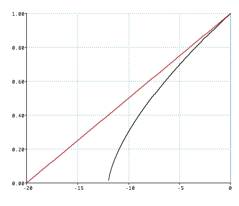
Note that even tho the scale factor increases monotonically, this has non-obvious consequences for distances: galaxy at a redshift z is at a proper distance
for "matter" including dark matter
\color{red}{\varepsilon _m \approx 1} GeV m-3
for vacuum energy,
\color{red}{\varepsilon _\Lambda \approx 2} GeV m-3
or in terms of Ω,
\color{red}{\Omega _r = 10^{ - 4} }
\color{red}{\Omega _m = .3}
\color{red}{\Omega _\Lambda = .7}
(we'll justify all of these later).
Can use this to answer various questions:
These have different scaling laws
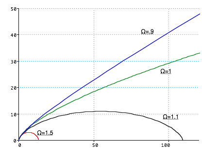
Multi Component Solutions
We have
\color{red}{
\left( {\frac{{\dot a\left( t \right)}}{{a\left( t \right)}}} \right)^2 = \frac{{8\pi G}}{{3c^2 }}\varepsilon \left( t \right) - \frac{{\kappa c^2 }}{{R_0^2 a\left( t \right)^2 }} + \frac{\Lambda }{3}}
More realistic universes are going to have 2-4 components. We'll follow Ryden in using Ω as the energy variable of choice:
Ωk,0 is the current value of the k'th density param:
\color{red}{
H\left( t \right)^2 = \frac{{8\pi G}}{{3c^2 }}\varepsilon \left( t \right) - \frac{{H_0^2 }}{{a\left( t \right)^2 }}\left( {\Omega _0 - 1} \right)}
or
\color{red}{
\frac{{H\left( t \right)^2 }}{{H_0^{} }} = \frac{{\varepsilon \left( t \right)}}{{\varepsilon _{c,0} }} + \frac{{\left( {1 - \Omega _0 } \right)}}{{a\left( t \right)^2 }}}
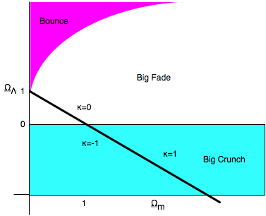
(Note \color{red}{\left( {\Omega _0 - 1} \right)}: will see that the nature of solution changes drastically if this is + or -).
Putting in the correct scaling laws, this gives us the general solution